Optimizing Multi-Band Wire Antennas

Simple pieces of wire are not the most sexy ham radio antennas, but they are probably the most ubiquitous, if for no other reason than that their cost-performance ratio is very good.  When it comes to the lower bands, there is little else that is more practical for most of us than using a wire antenna.  There are quite a number of wire antenna designs, promoted and sold by various manufacturers, but little discussion about what is really necessary to design a decent multi-band wire.  Any multi-band wire will be a series of compromises. Small variations in the design can make rather large changes in the optimum performance and “use profile” of a given antenna.  Antenna modeling is very helpful to finalize a design, but the key to using the modeling programs effectively is to understand which parameters matter, and for what.

Multidimensional optimization problems are always a challenge.  My approach is to first try to understand some of the physics and the expected trends in order to make a good initial guess for a solution.  Then we can use an antenna modeling program to verify performance and to suggest the best way to makes modifications that will result in better overall performance.

Factors Affecting Driving Impedance

Before we get into a detailed design, it is worth looking at the impedance properties for driven wires.  A few numerical experiments using the 4NEC2 antenna program can give us some insight.  When we are thinking about a multi-band antenna, this implies that for some bands there will be multiple wavelengths standing on the wire.  The figure below plots the impedance of a center fed dipole antenna in free space against the “wave number,”  where a wave number of 0.5 is the normal half-wave dipole with the expected impedance of about 72 Ω.  Note that as more waves are driven on the wire, the driving impedance goes up.  For a given current it takes more voltage to drive those additional waves.

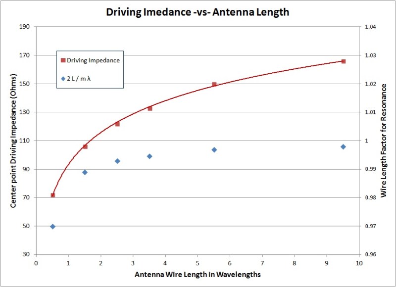
Also on the chart above the blue diamonds show the end-effect shortening that happens with wire antennas.  This is not a large effect, but it lowers the resonance of the fundamental more than the higher harmonics and adds to the difficulty of getting all bands to sing on the same length of wire.

Our antenna is not in free space but over ground.  So let’s look at what happens to the impedance when in close proximity to ground, here using 4NEC2’s “Average” real ground.  You can see that when the dipole gets close to the ground, the impedance moves around quite a bit. There are competing effects of the ground “shorting out” the antenna and generating ground losses and also the effects of driving a ground “image.”

I was surprised by the increase in impedance at around a height of 0.35 λ since the conventional wisdom is that the impedance drops for a low antenna, but as the simulations show – not always!

However, in general when we put these two effects together, what we discover is that a wire run on the lower band will have a lower impedance than the same wire run on a higher frequency band because of the ground proximity and the lower wave number on the wire.

One more effect worthy of a little simulation is off-center feeding and the change in driving impedance that comes when you do this.  The plot below shows how the impedance changes as the feed point goes from 1/8 to half-way along the wire length, as you move from the current maximum in the center, to the voltage maximum near the ends.

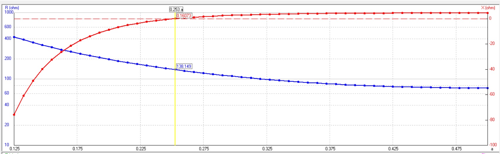
The right side of the graph is the center-fed case where the impedance is about 72 Ω.  The wire length was tuned slightly to remove the reactive component when fed at 1/4 of the way along the wire (yellow line) where the driving impedance is about 140 Ω.  So you can significantly change the driving impedance just by where you drive the wire.  This is an important tuning “knob.”

When the wire length is tuned perfectly to the operating frequency, the resonance condition implies that the feed point sees a perfectly resistive load.  Any mismatch will result in some residual reactive component to the load.  A wire that is too short appears capacitive, a wire too long will be inductive.  If you look at the Fig. 3 above, you can see that changing the feed location not only changes the real part of the impedance, but the reactive part as well (red line).  Similarly, changing the length of our mismatched transmission line can also give rise to the appearance of reactive terms in the overall driving impedance.  Our desired band center operating points for the various ham bands do not result in the exact same length of wire. Hence, we know there must be reactive impedance components that will need to be compensated.   The exact antenna length for the band, the off-center feed point, and the length of the mismatched transmission line will all give rise to reactive impedance terms that, if combined correctly, have a chance at producing “real” resonances on multiple bands.

The Process

We need to arrange the driving method to give us a good impedance match on the multiple bands where we would like to use the antenna.  This will require iterative parameter changes coupled with 4NEC2 model runs to help solve the multi-dimensional optimization problem.    For the impedance match problem, we need as many “adjustable parameters” as we can come up with in order to have enough “levers to pull” to optimize for multiple bands.  Here is what we can change for a simple wire:

1. Balun ratio.
2. Feed line impedance.
3. Feed line length.
4. Overall wire length.
5. Position of the feed point along the wire.

The first two items have only a few possible discrete choices.  Make an educated guess and proceed.  We could add traps and special circuit components to the wire to give us more knobs to turn, but I hope to convince you that this is already a pretty good set and will get you pretty far along.  The last three items are continuous variables, overall wire length, length fraction for feed position, and mismatched transmission line length, and they can all be varied in the 4NEC2 model program.  I will show a method that uses 4NEC2 to give you the information you need to converge on an optimum set of these variables.

Balun Ratio

If we have a 50 Ω transmitter, when you look at the graphs in Fig.1 & 2 above, you don’t see many points in the 50 Ω range (other than the very low dipole).  There is also no simple mechanism to reduce the impedance, but there is a simple way to increase the impedance by moving the feed off center.  Hence, an impedance step-up is called for.   I like current baluns that work best with simple integer turns ratios. A 2:1 turns ratio yields 4:1 impedance transformation.  A 50 Ω transmitter and feed will appear like 200 Ω to the antenna.

Feed-line Impedance

There is nothing in the books that says you have to feed your antenna with 50 Ω cable.  In fact the popular GR5V design uses a length of 300 Ω line as a matching section before switching to the 50 Ω cable for the run to the transmitter.  The purpose of the “mismatch” section is to generate reflections at both ends of the matching section that conveniently “cancel” each other out.  The matching section is nominally 1/4 wave long so that the reflected waves are exactly out of phase with one another.  If you want to use this anti-reflective technique to improve the impedance match you have to have a mismatched section of line.  In fact, the entire line can be a different impedance as long as the length of the feed line, between the mis-matches at the ends, is an odd multiple of 1/4 of a wavelength.  One can do well just using the balun and 50 Ω line to the transmitter, but doing so you lose one of the few tuning parameters that you have available which is the length of the mismatched transmission line. Hence, I’m going to advocate for using 75 Ω feed line for reasons you will see as we go along.

To have a perfect reflection cancellation with a 1/4 wave section of line the amplitude of the reflected waves from both ends must be the same, which imposes the matching requirement:

Where is the transmitter impedance,  is the antenna impedance and  is the transmission line impedance.  For a 50 Ω transmitter and 75 Ω 1/4 wave line, then the antenna impedance of 112.5 Ω would satisfy this requirement.  This is a simple method, without resorting to a balun or using a 1:1 balun to better match a multi-wave wire.  With the 4:1 balun, the best matched antenna impedance will be 112.5 × 4 = 450 Ω.  In this case the best off-center position will be quite far from center, as you can see from the graph in Fig.3.

Feed-line Length

The discussion above assumed that we had a nice 1/4 wave matching section, but this will be a problem when we are trying to make a multi-band antenna where we must accommodate several design wavelengths simultaneously. Remember, however, than any odd 1/4 wave multiple will have the desired properties.  And although it may not be possible to get exact cancellation of reflected waves, we can try to choose cable feed lengths that will at least tend to be helpful.  With that in mind, I created a table of the ham bands and the odd quarter wavelengths associated with the bands.  Then by trial and error I picked specific lengths of cable that approximately satisfy the odd quarter wavelength requirement.  The figure of merit was the residual fractional wavelength error for each band.  Several relatively good lengths popped out of the exercise, shown in the green boxes in the table below.

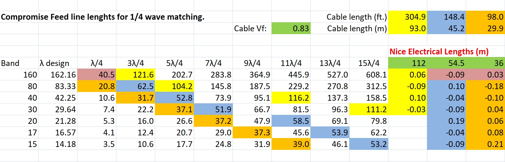
You have to be more accurate to the exact length for the shorter wavelength bands to get comparable errors across all bands.  Hence, slight changes in length will matter less on the low bands.  Consider the length of line in the green boxes as suggestions for a first-cut antenna design.  For a particular design we will optimize explicitly for the mismatch section line length.

Worked Example – Large Inverted V Low Band Antenna

We now have in our tool box several tricks that we can use to tune several bands on our wire antenna.  The best way to show the process in action is to work an example.  My current project is a large low-band inverted V that I would like to pull up into my tall trees.  I’d like it to work on 160, 80, and 40 meters – getting 20m would be gravy.

First look at the bands we want and the length of wire implied by each of them.  The electrical length less the end-effect shortening for desired band centers yields the lengths below.

160 m        1.860 MHz      λ/2 – 3%           78.2 m

80 m          3.760 MHz      λ – 1%               78.9 m

40 m         7.120 MHz      2λ – 0.5%           83.8 m

20 m       14.100 MHz      4λ                      85.0 m

Notice that the lower bands would like to have a shorter wire than the upper bands.  We will compromise at 81.5 m as our first-cut length.  If the model is including the effect of coated wire, such as is common with THHN house wire, then the length should be reduced about 4% because of the reduced velocity factor due to the coating.

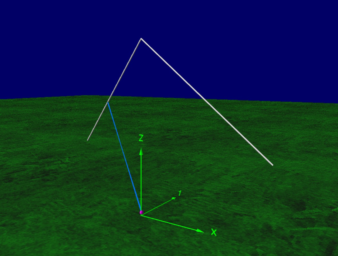
The basic geometry we will consider is an off-center-fed inverted V where we will also model the transmission line feed, as shown in the figure above.  As a starting point, I will assume a 4:1 balun and 54.5 meter electrical length of 75 Ω feed line.  We can begin optimizing the design using 4NEC2 for the overall wire length and the off-center feed point.  The NEC file is here for those who want to see how I set up the geometry with just a few free variables.

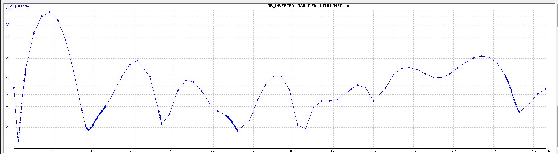
The first cut shows that the 4:1 balun is keeping the SWR pretty well constrained below ten just about everywhere that matters.  The off-center fraction was a total guess, so next step is to look at how the SWR varies with the off-center fraction for the various bands.

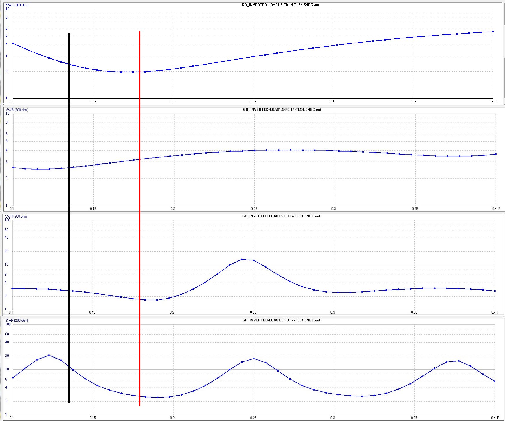
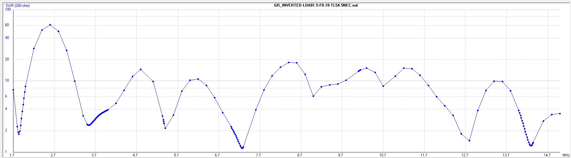
I chose band centers of 1.840, 3.760, 7.120, and 14.100 MHz for the four ham bands when I ran the sweeps above.  This is another choice you get to make for the optimization process.  From Fig.6 above,  we can see that increasing the off-center fraction from our initial guess will help quite a bit on 20m and 40m and only hurt a little on 80m, so that will be the next run, shown below.

Next we do the same kind of process again, this time running a sweep of the feed transmission line length at the desired band centers and see if there is anything more to be gained by changing that parameter.

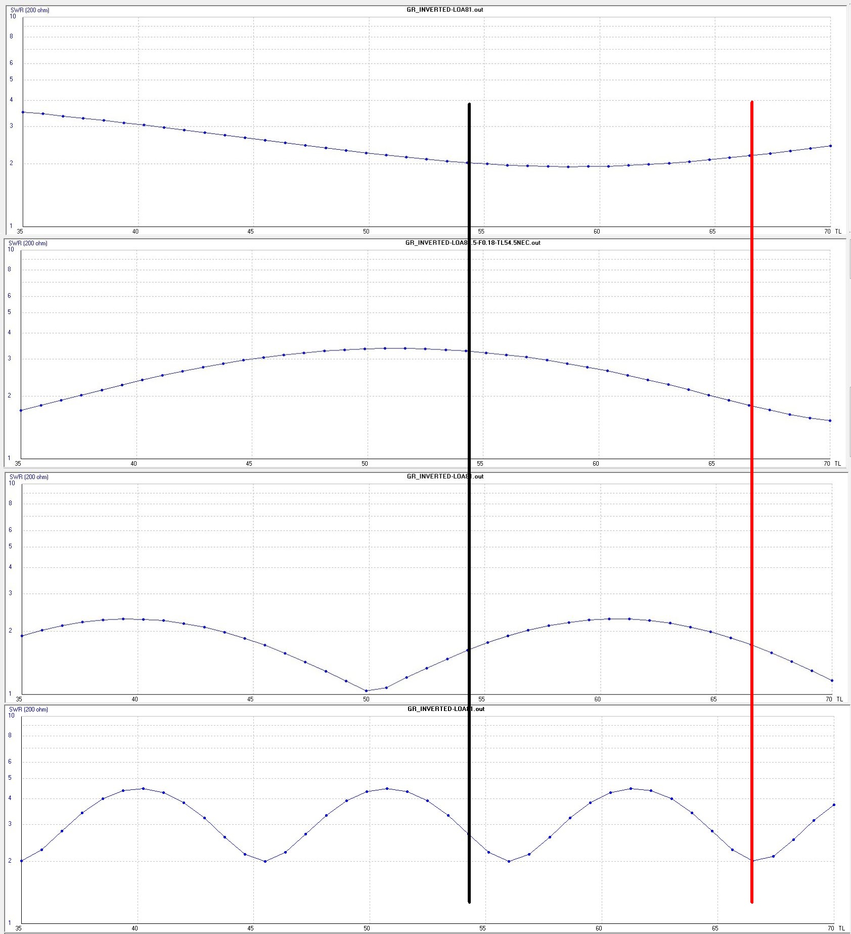
We make another educated tweak, this time to the transmission line length and then run the model again and see how it does.

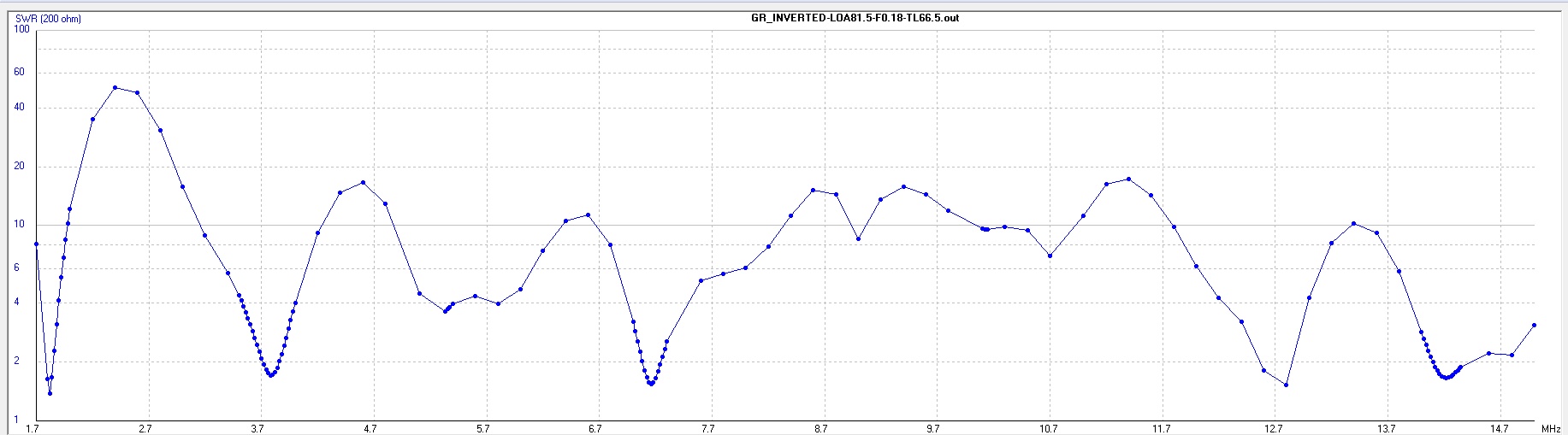
Not too bad.  One can iterate this process indefinitely, slightly tuning either the LOA of the wire, the off-center point, or the transmission line feed length after seeing how such a change would affect each band of interest.  At some point there will be little to be gained and you will either be satisfied with the design, or you will have to go back and adjust your goals or your overall approach.

There are some general problems that you will always face.  The low bands would like shorter wires than the upper bands.  Notice that even with our best effort above, 160 and 20 are resonant at the opposite ends of their respective bands, like we are trying to squeeze all we can from our fixed length of wire.  One very clever solution to this problem was proposed by Serge Stroobandt, ON4AA.  In his 80m “Center loaded” off-center-fed dipole, Serge inserts a small capacitance that can be used to compensate for the extra inductance associated with a longer wire, but one that is more happily resonant on the upper bands.  The trick with the “center loading” was to make use of the property that the higher bands were all even harmonics with a current null in the center of the wire.  At that location, the capacitor had little effect on bands where there was a current null, but would be part of the circuit on the odd harmonic bands, such as the 80m fundamental.  Stroobandt claims that this approach does not scale to the 160m antenna, but I’m not sure that is true.  The correct location for the capacitor would not be the center of the wire, but rather about a quarter of the way along the wire.  Adding this simple element would provide two more degrees of freedom to the design, with the position and value of the capacitor as the added variables.  I’ll leave it to the reader to take on that assignment and improve upon the design we developed here.