
There are quite a few recipes for building a suitable transformer for an end fed half wave antenna (EFHW), but I was never sure I really understood the main principles. So, I wound a bunch of transformers, made measurements on them using my NanoVNA, learned how to get what I really wanted out of the VNA measurements, and in the process discovered how to build better transformers and be able to predict what they will do. Here is the story.
One can verify with NEC models that, indeed as is conventional wisdom, an end-fed driving impedance of about 2450Ω works well to drive the antenna wire (see the companion post Engineering the EFWH 49:1 Transformer and Antenna). This implies a 49:1 impedance transformation from 50Ω, so a turns ratio of 7:1 is required for the transformer. Typical end-fed antennas are supposed to work on multiple ham bands, so the transformers must be broadband. The ferrite material characteristics will have a large influence over the frequency range where the transformer will perform well. For this application the NiZn ferrite mix 43 is often used because of its high resistivity and low core losses at high frequencies. I happened to have several cores of various sizes of this material, so this was the starting point for my investigations. Mix 43 has an initial permeability of about 850; the complete frequency dependence is shown below.

Ferrite materials become magnetized as the magnetic domains align to the excitation field. As the frequency of the excitation increases, there becomes a prominent phase delay in the alignment of the magnetic domains. Treating the permeability as a complex quantity includes this effect. In the chart above µ’ is the real part of the permeability, accounting for inductive reactance, and µ” is the imaginary part of the permeability where the phase difference generates a resistive component to the complex impedance. Notice that for the mix 43 ferrite, the crossover point for the real and imaginary components of the permeability is at about 7 MHz. The effects of this permeability phase shift will be important at the high frequency limits of our transformer. What drives transformer action is dB/dt, regardless of how you get the magnetic field B. At low frequencies the transformer primary appears inductive (with real µ’ dominant), so no real power is needed to establish the core magnetization. However at high frequencies where µ” > µ’, the magnetizing impedance will consist of both a reactive and real component, and real power will be dissipated in the process of establishing B. The transformer can still be useful as long as the magnetizing impedance is much greater than the load impedance seen at the primary.
A simple transformer equivalent circuit is shown below.
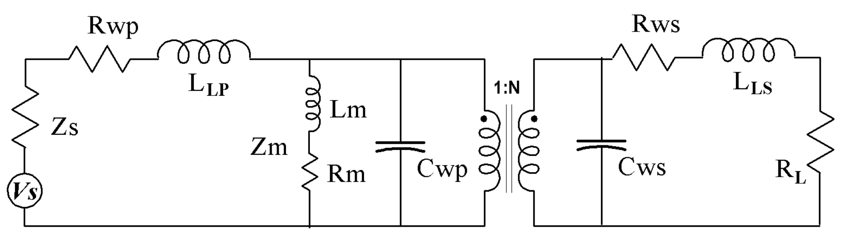
Besides the ideal transformer, there are leakage inductances LLP and LLS that result from imperfect flux coupling. The winding resistance for the primary and secondary are RWP and RWS respectively. The magnetization inductance, LM, is associated with filling the core with magnetic flux that is required for the ideal transformer action to take place. (Note that in the ideal transformer the amp-turns on the primary and secondary are exactly balanced so no net magnetic field would appear in the core.) Winding capacitance is modeled as Cwp and Cws. The secondary-side parasitic elements can be transferred to the primary side of the transformer, with appropriate scaling by the turns ratio squared, they can be combined with the primary-side parasitics. In the simplified primary-referred model below, CW = Cwp + N2 Cws ; and approximately RW = Rwp + Rws/N2 and LL = LLP + LLS/N2 .
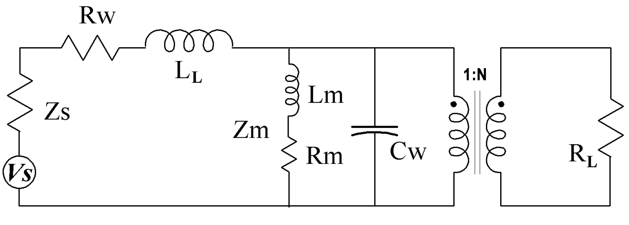
Core losses are lumped into RM and represent eddy current or hysteresis magnetic losses. For high frequency broadband transformers, wound with only a few turns of wire on high permeability cores, the leakage inductance and the series resistance of the windings will be small compared to the magnetizing inductance and the source impedance, respectively, so we can ignore these terms.
The low frequency cutoff will be determined by the source impedance and the magnetizing inductance,
fL= Zs/2πLM.
The high frequency cutoff will be determined by the source impedance and the combined winding capacitance,
fH= 1/(2π ZSCW) or by the self resonance of the leakage inductance LL and the winding capacitance CW.
With appropriate tricks, we can measure some of the more important parasitic elements of a transformer using a Vector Network Analyzer. I have one of the ubiquitous NanoVNA instruments that I used to characterize various test transformers.
Total Turns Experiment
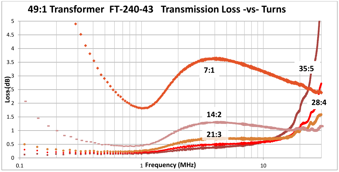
One question I wanted to answer was the optimum number of turns for a 49:1 impedance transformer. I wound several transformers on an FT240-43 core with 7, 14, 21, 28, & 35 total turns. The transformers were wound as auto-transformers with the primary tapped with a 7:1 turns ratio, so primary turns of 1, 2, 3, 4, & 5 turns respectively.
The table below lists some of the measurement results and calculated parameters for these transformers.
| Turns | LM+LL (µH) | LL (µH) | RW (Ohms) | Open Circuit SRF (MHz) | Open Circuit SRF Rmax (Ohms) | Core AL (µH/n^2) | LM (µH) | CW (pF) | LM 50Ω LF Cut-off (MHz) | CW 50Ω HF Cut-off (MHz) | LL CW HF Cut-off (MHz) |
| 7:1 | 1.19 | 0.175 | 0.09 | 23 | 65 | 1.015 | 1.015 | 47 | 7.84 | 67.5 | 55.4 |
| 14:2 | 4.45 | 0.409 | 0.11 | 7.92 | 185 | 1.010 | 4.041 | 100 | 1.97 | 31.9 | 24.9 |
| 21:3 | 9.82 | 0.795 | 0.137 | 4.41 | 362 | 1.003 | 9.025 | 144 | 0.88 | 22.1 | 14.9 |
| 28:4 | 17.4 | 1.33 | 0.197 | 3.17 | 648 | 1.004 | 16.07 | 157 | 0.50 | 20.3 | 11.0 |
| 35:5 | 27.6 | 1.87 | 0.112 | 2.28 | 1145 | 1.029 | 25.73 | 189 | 0.31 | 16.8 | 8.5 |
Here is how I got the above numbers using the NanoVNA. With the calibrated instrument, an S11 sweep was made into the primary of the transformer with the secondary open, and once again with it shorted. The NanoVNA Saver software is happy to plot the equivalent series inductance obtained from the S11 measurement. I recorded the low frequency effective inductance found at 500kHz for the various configurations. With the secondary open, the quantity recorded was LM+LL. With the secondary shorted, then only LL is measured. The frequency sweep shows a distinct resonant peak where the winding capacitance resonates with the primary inductance. Measuring the self resonant frequency (SRF) allows us to determine the winding capacitance CW.
For the next step I connected the network analyzer’s S21 port to the secondary of the transformer through a 2400 Ω resistor (it was actually 2469 Ω). The resistor and the analyzer’s input impedance provide a nominally matched load for the 49:1 impedance transformation in the transformer. The S11 reflection can tell us the VSWR of the transformer with the resistive match. The figure below shows the VSWR plots for the five transformers.
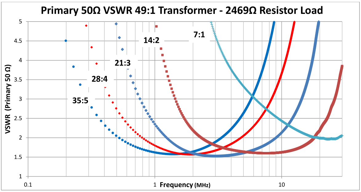
The lower cutoff frequency based on the primary magnetization inductance qualitatively matches with the increase in SWR on the low end. The winding capacitance interacting with the leakage inductance may be mostly responsible for the limitations at the high frequency end, but also bear in mind that the ferrite is exhibiting its complex behavior above 7 MHz. We can get a better handle on this by seeing what is going through the transformer.
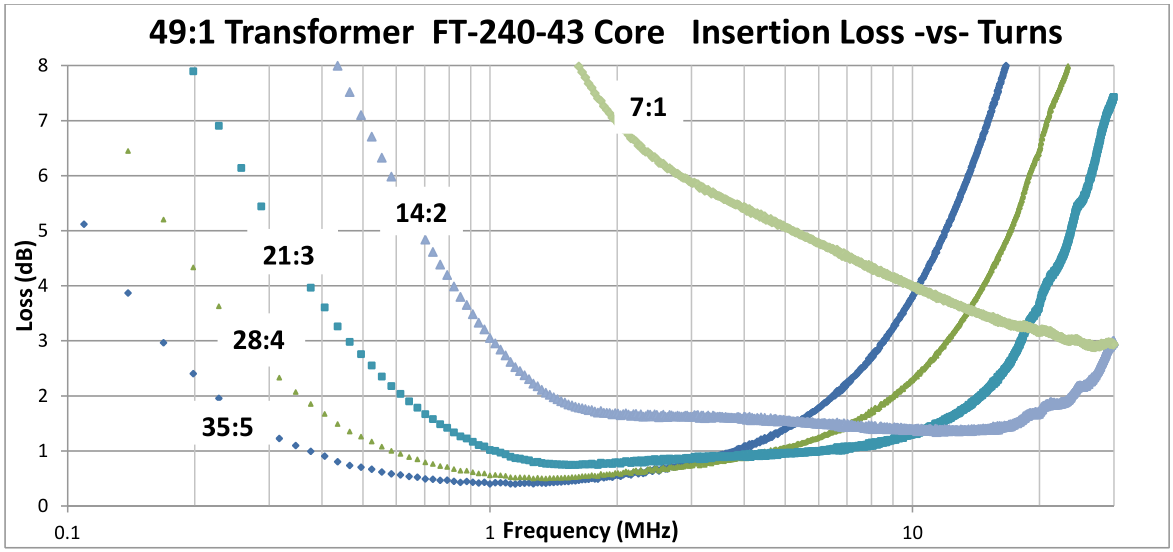
Now we are getting to the crux of the matter as core losses shows their colors. The measurements show that the even in the middle of the transformer pass band, more turns means lower losses. Note that the B field in the core is inversely proportional to the number of turns. Faraday’s law says that V = -N dΦB/dt , the driving voltage per turn of the circuit is proportional to the rate of change of the magnetic flux. So for more turns, the same driving voltage waveform generates less magnetic flux. Ferrites made of NiZn have a very high resistivity which means the eddy currents are almost non-existent and the magnetic field penetrates the entire volume of the material. However, hysteresis losses are proportional to the B field level in the core, so one would expect that core losses from this mechanism would decrease proportionally to the number of turns. At least roughly qualitatively, that is what we see.
Core losses will generate heat in the core material. The Insertion Loss plotted above also included losses that come about because some of the incident waveform is reflected back to the source. Once you correct for this effect you can plot the Transmission Loss which can be equated with heating in the core. This even more clearly shows that the losses are inversely related to the number of primary turns.
Core Loss Models
What goes on inside the ferrite material as it cycles through magnetization excitation is not well represented analytically in any information that I could find. Qualitatively, as the core is cycled around an open hysteresis loop, the stored energy represented by the flux inside the open loop is lost to heat for each cycle of the field. A common simple empirical power law model for ferrite losses, Ploss, includes the basic features you would expect from this qualitative understanding:
Ploss = k1 fk2 Bk3
where k1, k2, and k3 are the fitting coefficients, f is the frequency and B is the magnetic field strength. The literature for power loss in ferrite transformers for power switching applications finds the frequency exponent k2 between 1.3 and 1.9, and the magnetic field exponent k3 between 2.5 and 2.9 depending upon the paper and the experiment.
The energy stored in the core at peak current can be written in terms of the inductance and the current, or in terms of the magnetic field energy density and the core volume V.
Ecore = L I2/2 = V B2/2µ0µ
If a fixed fraction of the core energy is lost each cycle, that would give rise to a direct frequency dependence for the power loss, k2=1. Similarly, with the B2 dependence on the stored energy, losing a fraction of of it would give rise to a B2 dependence for the power loss, i.e. k3=2.
If k3 is larger than 2, as reported in the literature I found, then it would seem that the overall power loss would decrease if you traded B field intensity for volume while maintaining the same inductance and current.
Core Size Scaling Power Loss Experiment
The considerations above led to an experiment where I wound several transformers on cores of different sizes while adjusting the number of turns to obtain roughly the same primary inductance. Below is a table that shows the characteristics of the test transformers.
| Core | N primary | N Total | Lprimry (µH) | LLeak (µH) | Cp (pF) | Fsr (MHz) | Core Area (cm2) | Core Vol. (cm3) | Core Mass (gm) | Len. Wire (mm) | Calc. µi | 3.0 MHz Trans loss (dB) | 3.0 MHz Loss % | Loss Corr. for Lprimry |
| 2xFT240 Mix 43 | 2 | 14 | 8.4 | 0.46 | 133 | 4.77 | 3.16 | 45.6 | 248 | 1055 | 773 | 0.638 | 13.7% | 13.2% |
| 1xFT240 Mix 43 | 3 | 21 | 9.5 | 0.72 | 133 | 4.53 | 1.58 | 22.8 | 124 | 1055 | 778 | 0.577 | 12.4% | 13.6% |
| 4xFT114 Mix 43 | 2 | 14 | 8.04 | 0.3 | 88 | 5.98 | 1.48 | 10.8 | 56 | 969 | 809 | 0.730 | 15.5% | 14.3% |
| 2xFT114 Mix 43 | 3 | 21 | 9.3 | 0.41 | 83 | 5.72 | 0.74 | 5.4 | 28 | 832 | 831 | 0.657 | 14.0% | 15.0% |
| 1xFT114 Mix 43 | 4 | 28 | 8.22 | 0.49 | 68 | 6.73 | 0.37 | 2.7 | 14 | 694 | 827 | 0.756 | 16.0% | 15.1% |
| Ave: | 8.69 | (µH) | Loss stdev | 1.4% | 0.8% | |||||||||
| +/- | 9% | Max | ||||||||||||
| SMLCOR | 2 | 14 | 7.82 | 0.21 | 100 | 5.69 | 1.6 | 11.28 | 54 | 711 | 600 | 0.482 | NA | NA |
| FT240_31 | 2 | 14 | 7.88 | 0.36 | 119 | 4.41 | 1.58 | 22.8 | 124 | 703 | 1451 | 1.483 | NA | NA |
| 3E2A | 1 | 7 | 8.16 | 0.13 | 4290 | 0.85 | 1.24 | 9.51 | 45 | 315 | 4533 | 4.959 | NA | NA |
Core mass was varied from 248 grams to 14 grams, changing the winding numbers to keep the primary inductance as close to about 8.5 µH as possible. Measured with the secondary open were the primary inductance and the self resonant frequency to be able to derive an equivalent primary-reflected winding capacitance. With the secondary shorted the primary leakage inductance was measured. Both measurements were made a 500kHz. From the inductance and the coil geometry it was possible to calculate the core relative permeability. Mix 43 ferrite is supposed to have µi~850. The two large cores came in at about 775, and the small cores at about 820. The large and small mix 43 cores were purchased at different times from different places, so some variation in batch parameters is to be expected.
All transformers were wound with tripled #28 enameled wire. I have a big spool of this wire, which is a little on the small side, but tripled and given a twist it is a reasonable overall size and handles well during he winding process. Winding resistance, just a few milliohms for the relatively short lengths of wire needed, is not a significant loss mechanism for these transformers.
Loss measurements were made on each transformer as was done above in the total turns experiment and as described in the appendix. The graphs are shown below:
I was surprised by how little spread there was in the loss characteristics for cores ranging over a factor of 20 in core volume and mass. Almost half of the observed variation in losses in the mix 43 cores can be explained by the fact that the primary inductance varied by +/- 10% because of the quantization imposed by a full turn of the winding. When the losses were corrected linearly for this inductance variation, the deviation in the results dropped even further. The table includes the observed loss at 3 MHz and the corrected losses based on the difference in measured primary inductance from the average.
This rather surprising result says that if you are worried about transmission loss, the only remedy is a higher primary inductance. Total heating power will be pretty much the same whether you are using a 250 gram core or a 14 gram core! Obviously a larger core with more surface area may be able to convect the heat away more effectively than a small core, but the larger core otherwise has no particular benefit.
It should be noted that the excitation level in the core supplied by the NanoVNA measurement is very small compared to the levels used in typical applications. The NanoVNA excites with about a 2mW into 50 Ω square wave. The B field level in the core at 3.5 MHz varies from about 0.03 mT using two FT240’s to 0.14 mT with the single FT114 core. But these levels are far below the saturation level, 350 mT, or the recommended flux maximum working level, 200mT, for type 43 ferrite. If nonlinear effects show up at higher flux levels, our experiment would not have detected them.
Core Material
My investigations centered around mix 43 NiZn toroids because these are what are very often recommended for HF transformers and I had a selection of these cores on hand. I also had several other cores of various ferrite mixes on hand including some large FT240-Mix-31 cores, a couple of compact NiZn cores of unknown origin, 1.38″ O.D. and 0.38″ I.D., which I’ve called SMLCOR, and a low frequency, high permeability, Ferroxcube 3E2A material MnZn core.
Again I built transformers from the cores of these other materials such that the primary inductance was as close to 8µH as I could make it. And again I measured the primary inductance, leakage inductance, and losses using the NanoVNA. The characteristics of these transformers are listed in the last three rows of the table. The chart below compares the transmission loss for transformers made with these various core materials.
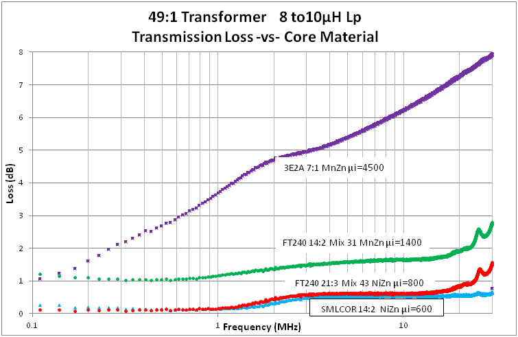
Clearly the high permeability MnZn ferrite is unsuitable for this task – but we knew that. One thing we can see is that the MnZn ferrites show a much stronger frequency dependence than the NiZn samples. This is more in line with the core loss model mentioned earlier where a frequency power law exponent of >1 is expected. In contrast, the NiZn ferrites show roughly constant losses over about three octaves in mid-band frequency. The mystery SMLCOR proved to be the lowest loss material, still flat at 30 MHz. I wish I new how how to get more of it! In retrospect, I believe the origin of that core was a sample for evaluating the material as a “kicker” magnet at the Indiana University Cyclotron Facility were I worked for a few months.
Compensation
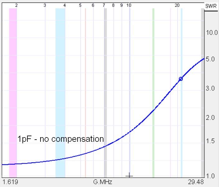
The low frequency performance of these transformers can be quite good with sufficient primary inductance. However, a large primary inductance implies more total turns and higher winding capacitance which limits the high frequency performance. Often there are tricks to play to increase the high frequency pass band and the expense of a stronger even higher frequency roll-off. Before we begin, it is a good idea to have some idea of how much primary-reflected capacitance is going to be a problem at, for example 25 MHz. The 50 ohm capacitive reactance implies:
50Ω = 1/2πfC ==> C = 127pF for f = 25 MHz
If you glance at the table above with the measured transformer characteristics, you will see that the primary-reflected capacitance, as determined from the observed self resonant frequency, falls in this ball park. The best thing to do is to try and reduce this capacitance by spacing the windings out and keeping a distance between start and finish ends of the winding, keeping other conductors away from the winding and nearby dielectrics low, etc. But with the high impedance ratio of the transformer, just a couple of pico-Farads of secondary capacitance will show up as ~100 pF at the primary. Hence, the high frequency performance will always be a challenge.
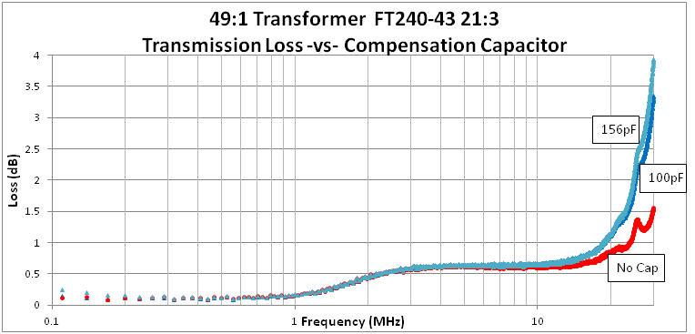
I found the SimSmith program to be very handy to see what is going on when applied to a primary-referred circuit model. Below is the SimSmith model that uses the leakage and magnetization inductance and the primary-referred capacitance obtained a 500kHz for the FT240-43 21:3 transformer that we used in the studies above.
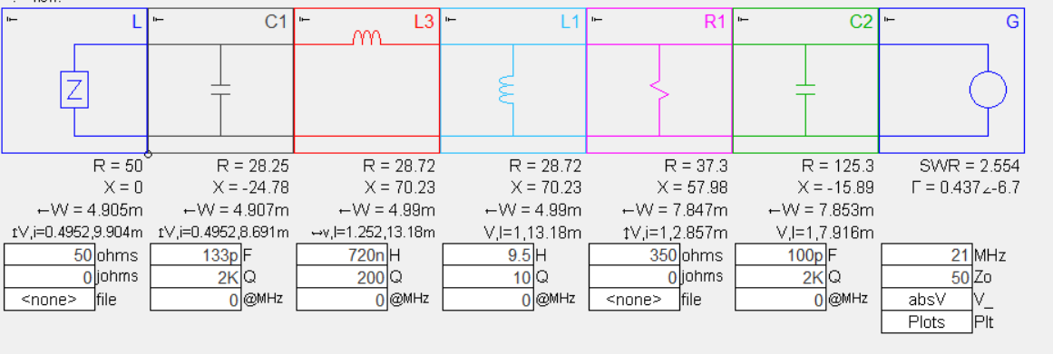
The capacitor C2 on the generator-side is the compensation capacitance. (SimSmith works from the load on the left to the source on the right) For high frequencies L1, the magnetization inductance, can be ignored and we are left with a little pi network consisting of the winding capacitance, C1, the leakage inductance, L3, and the added compensation capacitor C2. The figure below shows the effect of adding capacitor C2.
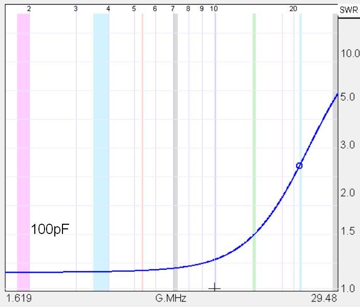
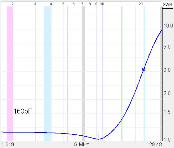
Let’s not be satisfied with just theory. We can look at the actual SWR plots for our test transformer, shown below.
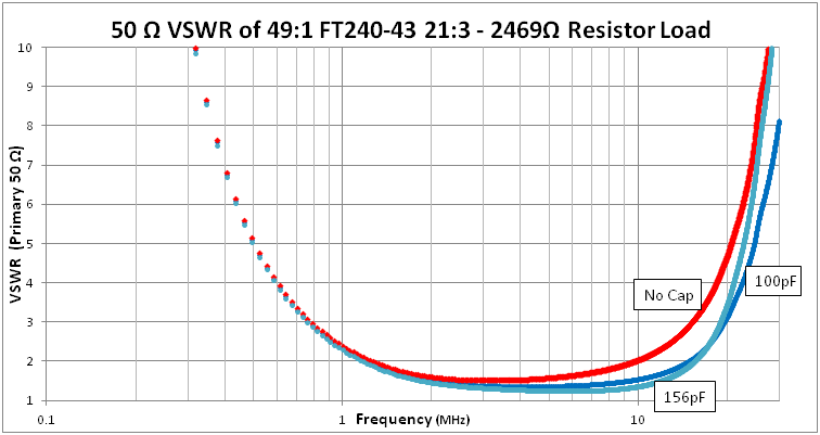
Qualitatively we see the same behavior as with the SimSmith model. However, the upper end cutoff seems to be coming a little lower infrequency. Most likely this is because SimSmith knows nothing about the nonlinear core material we are dealing with which rears its head above 10MHz. In fact, it you look at transmission losses which include the compensation capacitor, you discover that the capacitor enhances core heating at the high frequencies. The better match of the source provided by the compensation capacitor allows more energy to be delivered to the core rather than reflected back to the source. We have a double edge sword here!
After initially releasing this post, I was made aware of John Oppenheimer, KN5L, and his EFHW transformer design and analysis. It is a perfect example of extending the lessons learned here to a practical design. Rather than a physical compensation capacitor, the KN5L winding method enhances the distributed primary winding capacitance by winding the first part of the secondary back on top of the primary turns. The close coupling of primary and secondary also significantly reduces the leakage inductance. He uses two FT114-43 cores with 4 primary turns to get ~16 µH primary inductance and low loss.
Discussion
Ultimately the ferrite material properties imposes limits on the performance of these transformers. Looking at the permeability plot again, the mix 43 material is quite obviously going to have trouble above 20 MHz regardless of what kind of tricks you play. Transformers wound with enough primary turns to keep mid band losses low, start to lose it once the core permeability degrades at high frequencies.
Compact cores make better transformers. The core size experiments explored a lot of parameter space besides core volume. If you define the core aspect ratio as the magnetic length divide by the cross sectional area, you will discover that fat little cores with small holes do better than bicycle tire shaped cores. The benefits of low aspect ratio include, 1) more inductance per turn so you get the desired primary inductance with less wire. This usually means, 2) less winding capacitance, as long as you can maintain a little separation between turns in the center of the core. And 3) lower leakage inductance is natural with the shorter magnetic path length. A good example is to compare a single FT240 core with the SMLCOR (see table). Both have the same cross-section area but the SMLCOR has about half the magnetic path length. Despite a lower permeability, the SMLCOR achieved the desired primary inductance with just 2 turns whereas the larger mix 43 core required three turns. Hence, the SMLCOR had 1/3 less winding capacitance and more than three times less leakage inductance than the FT240 core. The main downside to a core with a small hole is that the inside section of the core will see more field intensity than the outer section. If you are operating at high field intensities, saturation will happen first on the inside radii.
The lessons learned here can be lead to a rather different looking transformer. See the companion article, Engineering the EFWH 49:1 Transformer and Antenna, for an example.
Appendix
The plots here were made from data obtained from a NanoVNA. The NanoVNA Saver software lacks the capability to make the plots and data manipulations that were required so the NanoVNA data was imported into Excel and manipulated there. The NanoVNA provides Frequency, Re (S11), Im (S11), Re (S21), and Im (S21) as space delimited data for each frequency point in the “.sp2” files you can save in the NanoVNA Saver software..
The insertion loss of the nominal 2400Ω resistor was measured with the NanoVNA with the resistor between S11 and S21 ports of the analyzer in a separate calibration procedure. The normalized power transmission through the resistor is given by:
Tres = |S21|2 / (1-|S11|2) and TresdB = 10 Log(Tres)
Note that by doing this calibration through the resistor, the absolute value of the attenuation and termination resistor is not critical. Resistor errors from the ideal may change the VSWR, but will not give rise to errors in the through-put (S21) quantities.
For the transformer tests, the following derived quantities were computed in the spreadsheet.
|S11| = Sqrt[Re(S11)2 + Im(S11)2]
|S21| = Sqrt[Re(S21)2 + Im(S21)2]
VSWR = (1+|S11|)/(1-|S11|)
Insertion Gain = |S21|2 / Tres and Insertion Loss dB = -10 Log( |S21|2 / Tres )
Transmission Gain = |S21|2 / [ (1-|S11|2) Tres ] and Transmission Loss dB = -10 Log(Transmission Gain)

Excellent article. Ham radio needs more li it.
Renee KC3NG
Outstanding as usual!
Have you ever thought about playing around with magnetic loop antennas? Similarly to EFHW, they require an intense level of electrical engineering fundamentals to have any hope of understanding (which is why I don’t really understand them). I know enough to know that the essential idea of resonating with ultra-low impedance and thus exceptionally high current and voltage (at 100W) make it incredibly challenging to build them to handle a standard 100W rig. But what about QRP? It appears to me it should be possible to build relatively low cost magnetic loop antennas even for 160m band for not *too* much cost if the power is kept low, but I haven’t really seen such designs out there. The really astonishing thing is that they only need to be one loop diameter above the ground to work well, unlike wire antennas which need to be 1/2 wavelength above the ground to work well. For 160m and 80m that is a huge deal.
I have played around with EFHW while traveling, but even though they are easier than a dipole, it’s still a pain to get them high enough on 40m which is the best band the past few years. The biggest challenge for magnetic loop which can travel is that anything which makes it more portable generally also increases the resistance. Also, the commercially available portable designs are basically worthless on 160m and 80m because the loop size is much too small. They’re optimized for 20m and the range of frequencies is not nearly as much as the sellers claim.
Daniel
Hi Daniel,
A couple years ago our club did a magnetic loop antenna project build. Strictly QRP, they used air variable capacitors. The capacitor is the hard part. The more voltage it can handle, the more power you can run. Other than that, there is not much to them — I highly recommend that you dig in and see what happens! Start simple, build it yourself, make lots of measurements, WSPR, FT8 and PSK Reporter, etc. to see how well you can be heard, questions will come and pretty soon you will be the expert!
Very informative, it’s nice to see nicely presented information like this.
It’s greatly demystified transformer design for me! I muck around with 5-1 and 9-1 alot for “random” wire antennas and this helps.
Excellent information with real details! Thanks for that!
Just wonder what exact difference it makes, to twist the primary coil (the one to the coax) with the secondary.
It’s my understanding that the energy transfer is based on a magnetic coupling, like it happens in any other
transformer. So – why did the initial designer (inventor?) of the EFHW antenna rumors showed us his twisted wires
and everybody is doing the same ? I built and measured a 1:49 by just tapping the second of 14 turns – it works!
73s, OE1MWW (3 times as 8Q7WK, last time with an EFHW)
Hi Wolfgang, I was suspicious of “black magic” when I first saw the recipe for the twisted turns. You do want to minimize leakage inductance, but the best way to do that is with a tap soldered to the wire. The other bit of “black magic” is the reverse halfway through the secondary to wind it back the other way. Very little good reason for that either! Stray capacitance and inductance do dominate the performance at 10meters and up, but the common construction methods are not necessarily the best way to tame them.
Will you be going to the Maldives again? That is still one of those places that I’ve never talked to.
Cheers,
Gary AF7NX
Hi Gary, yes ‘black magic’, for twisting and cross-over, that’s the right word. As for the Maldives – 2018 was a little bit disappointing, due to specific weather condx end of 2016 they had a coral bleaching again in that area. Holiday operation: I used QRP all the time as 8Q7, last time operating FT8 only, but that was not so bad ;-) Maybe we will go again in a few years, my 3/8 for 20m (QST 04/2019, page 44) is ready and sunspots will hopefully be high up. The 3/8 for 20m fits better on a 10m mast, Radiation efficiency EFHW 3/8 still to be compared ???. The EFHW for 20m was a little bit tricky to mount, needed an ‘extension’ on top of the 10m mast. (transport dimension: 67cm / 26″, extends with 13 elements) 73s, Wolfgang
I have my own EFHW winding design covered in this paper:
https://drive.google.com/file/d/0BwFicJLV0O4jWDNVZGN5S0FXeXc/view?resourcekey=0-vuul5TIrY-nr6HX9n5y8lg
As well as a circuit model for EFHW transformers which I used to calculate losses to a multiband antenna
https://drive.google.com/file/d/0BwFicJLV0O4jNWJrcDFvWlh5OG8/view?resourcekey=0-sS98PSV0tRzO1MZKnp8Lhg
I used various amounts of flux leakage to try to match what might actually be measured from a transformer.
Hi Daniel,
I saw your innovative design when I was researching this project. The main reason I went along a different track is that I felt that reducing the leakage inductance was important when trying to generate a wide-band device. Your approach was more to properly compensate for the leakage inductance you ended up with — (correct me if I’m wrong). I like your analogies with plucked strings!
I really like your thorough analysis of the transformer and the number of windings. The only thing I would add is that in practice, it seems that achieving an efficient radiator with a EFHW antenna is an interaction between the reactance of the transformer and the antenna. The capacitance (especially secondary capacitance, even only a few pF) at the higher bands (10 m) actually helps the antenna match. If the antenna is slightly shorter than the harmonic length, then it is inductive, and in parallel resonance with the capacitance of the transformer secondary, both helps to cancel the reactance and increase the impedance of the load which helps match the antenna. At the higher bands, the impedance of the wire drops with harmonic number, even to as low as 600 to 1000 ohms of resistance at 10 m for an antenna with 80 m fundamental frequency, which ought to make the match poor, but the parallel resonance effect boosts the impedance and improves the match.
This is why at the higher bands the match to a 2500 ohm load is not necessarily what is required to achieve a matched load. I used a model based on the induced EMF model of the antenna feedpoint impedance, but it had to be modified to accommodate losses from copper/radiation at half wave frequencies.
Having looked in a myAntennas transformer and seen the potting, the dielectric constant of the potting in between the turns of the transformer must increase the capacitance of the secondary winding. I would guess there might be as high as 5 pF of secondary winding capacitance for the transformer (which for 49:1 could be the “equivalent” of 250 pF or so). Most of this could be figured out by attaching short/open/matched loads to the myAntennas transformer and looking at the impedance looking in to the transform to characterize its two port transfer function.
Hi Daniel, I agree that there is much going on with the interaction between the wire and parasitic L and C in the transformer. If you think about where the C stray is located, it can be either before or after (or both) the “equivalent” leakage inductance. With the leakage inductance very small – it seems like the only parasitic you are left with to worry about is the output capacitance. If the leakage inductance is larger, then that L is the bottleneck at the high frequencies and building a little piece of equivalent transmission line from C_comp L_leakage and C_out seems to work OK. I’ll just say that by keeping the leakage inductance very low, you have more options! There was actually a modestly OK SWR at 6m in the device I presented. I didn’t test it there — but just goes to show that you can gain significantly in the useable bandwidth by controlling L_leakage. But you are absolutely correct that you have to include the wire in the final “equivalent circuit.”
Hello, Gary, fantastic piece of information. I wonder if you would allow me to publish a translation of this article on radioamator.ro, the unofficial ham radio website for romanian hams. Looking forward, 73 de YO3ITI Miron
Please do. Thanks for asking!
Nice analysis