
After doing the ferrite transformer scaling experiments last time, and learning a bit more about what matters in these transformers, it was time to make a stab at designing one. Let me review the salient observations from the previous work. 1) More primary turns and primary inductance improve the transformer efficiency and low end performance. 2) Winding capacitance and leakage inductance, especially present as you increase the number of turns, limit the high frequency performance. 3) Total losses are approximately independent of core volume. Other observations along the way: 4) Tight windings or backwinding over the primary can significantly reduce leakage inductance. 5) It is very hard to avoid stray capacitance on the output.
I don’t have an amplifier, so only need to be able to handle 100W. With most operations you only transmit for 50% of the time, and since a small transformer with four or more primary turns can achieve >90% efficiency, that implies that I really only need to dissipate ~5W. Gut feeling says that should be possible with just a couple of FT114-43 cores, similar to the design by John Oppenheimer, KN5L. My concern with the KN5L design is mostly about voltage breakdown through the enamel insulation where the secondary crosses the primary ground. Even at only 100W, the RF voltage on the high Z output of the transformer can easily be >1300 Vpp, so this is not an idle concern.
Transformer Construction and Electrical Characteristics
If you want to minimize leakage inductance, the way to do that is to keep the two windings very close to one another. However, to minimize capacitance, you want to spread turns and keep windings apart, so what is the right approach? I wish I had a simple answer, but really this is where some experimentation can pay off. I settled on a compact secondary using #28 wire. With the entire winding length short, the flux from the primary need not travel all the way around the core to link all of the secondary turns. To further improve the flux linkage, I wound the primary on top of the secondary. To mitigate the voltage issue mentioned above, I used a couple layers of Kapton tape over the secondary winding.
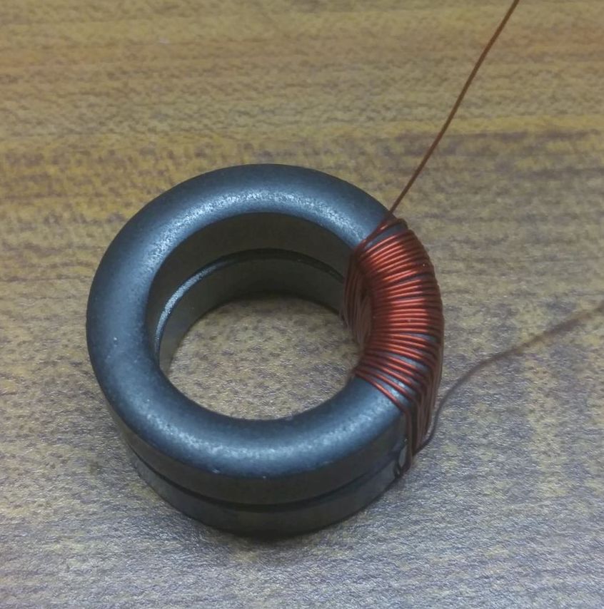
The photos above show a method that works fairly well. I decided to push for best efficiency with a 5-turn primary. Thirty turns #28 are wound on the two FT114-43 cores. Two layers of 1mil Kapton tape are placed over the winding. The low end of the secondary, which will be the tap, is bent back over to the center of the winding and covered with a small piece of Kapton tape, and then the primary is wound over the tape (and the secondary tap wire). I used four parallel #28 wires (not twisted) for the primary. The five primary turns cover about 60% of the secondary winding, leaving the high-side of the secondary not covered. In practice, exactly how you wind the primary turns can drastically affect the high frequency behavior of the transformer when measured into a 2450 Ω load. What seemed to work best was to concentrate the turns on the tap-side of the secondary winding, using several (#28) wires in parallel for the primary turns such that they covered about half of the underlying secondary winding. On the ends of each winding I slip the end under the last turn and pull tight to lock the winding in place. Tap and primary high-side are soldered together near the middle of the secondary winding; the ground side of the autotransformer is located over the low-end of the secondary turns.
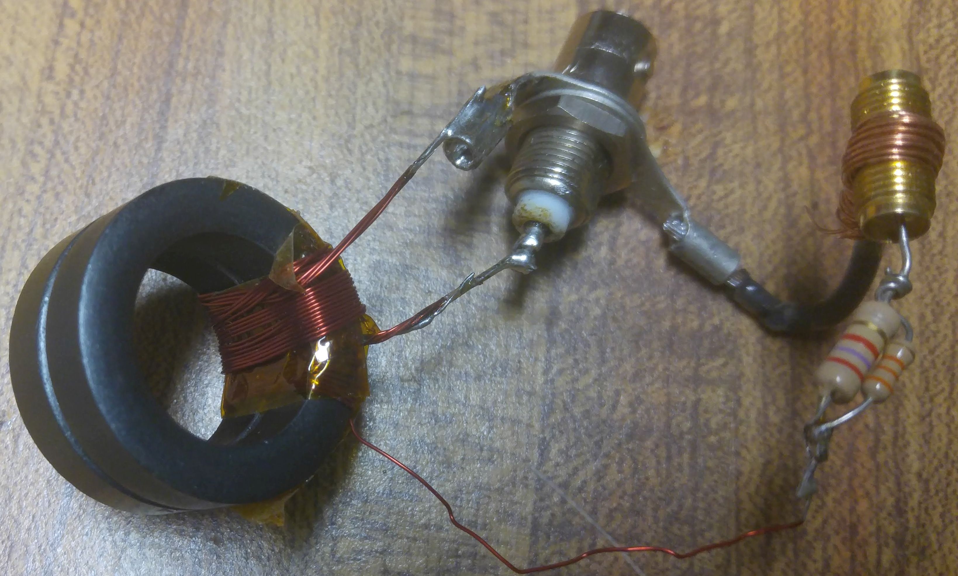
Measurements were made on the unmounted transformer with just a ~2 inch length of lead from the secondary to the 2450 Ω load and sampling resistor (jig connections as shown in the photo above). The high frequency performance was extraordinarily sensitive to anything that could add capacitance to the output lead.
Let’s do a quick calculation to see how much an issue is this output capacitance. Consider the RC time for a source with 2500Ω impedance into a 1pF capacitor. RC = 2500 x 1.0e-12 = 2.5 nS Now consider the period of a 30 MHz wave. τ = 1/30.e6 = 33 nS. For a “quarter wave” that is about 8 nS. Hence after about 3pF of output capacitance, the source will have a hard time charging up that capacitance before it is time to start discharging it. This totally un-rigorous calculation just gives a quick idea of how much you have to be careful. In this case, it looks important.
| Inductance (µH) | SRF (MHz) | Cp (pF) | Cs (pF) | Secondary | Set-up |
| 0.198 | 41 | 76.1 | 1.6 | Shorted | Primary Leakage Inductance |
| 25.8 | 2.43 | 166.3 | 3.4 | Open | #28 straight 2″ & resistor |
| 25.8 | 2.54 | 152.2 | 3.1 | Open | #28 straight 2″ No resistor |
| 25.8 | 2.72 | 132.7 | 2.7 | Open | #28 folded twice 1/2″ |
| 25.8 | 1.59 | 388.3 | 7.9 | Open | 18″ clip lead |
| 25.8 | 1.83 | 293.2 | 6.0 | Open | Mounted in Aluminum Box |
| 25.8 | 1.77 | 313.4 | 6.4 | Open | Boxed w/resistor |
It turns out that we can easily measure the effective parallel secondary capacitance by looking at the primary self resonance when the secondary is open. See the table above. Because of the turns ratio N, the secondary capacitance will appear N2 larger at the primary and will resonate with the primary magnetizing inductance. When you are discussing a distributed capacitance, it is difficult to know exactly what you are measuring. The smallest number I measured was 1.6 pF, derived from the self-resonance at 41 MHz with the leakage inductance (measured at 198 nH) when the secondary was shorted. The second smallest number I measured was 2.7pF, derived from the self resonance at 2.72 MHz with the magnetizing inductance (measured at 25.8 µH) with the secondary open and the output wire folded to a small 1/2″ length.
When the transformer was mounted in its box and the output connected to an antenna connector feedthrough, the observed capacitance increased dramatically to about 6.0 pF. For fun, I attached an 18″ clip lead to the secondary output and observed 7.2 pF due to the dangling clip lead. Which begs the question — what happens when you attach the antenna? We will return to that shortly, but first let us look at the VSWR associated with such added capacitance when driving the 2450 Ω load resistor. The VSWR plots below show results from the same transformer tested on the bench with minimal output capacitance, with a primary “compensation” capacitor, either 100pF or 27pF included, with the transformer installed in it’s aluminum box including antenna connector feedthrough, and with the transformer with an 18″ clip-lead on the antenna output.

The commonly used primary compensation capacitor does not work very well for this winding method which keeps the leakage inductance as low as it does. It is clear that the capacitance from just mounting the transformer in it’s box generates a significant reflection at 30MHz for the 10 meter band. However, from the measurements we made on the self resonance frequency, we know that most of this capacitance is right at the output of the transformer and not internal to the windings. To compensate for the antenna connector capacitance, the solution might be to add the appropriate inductance “on the wire” right near the box.
The impedance per unit length of a lumped transmission line is 
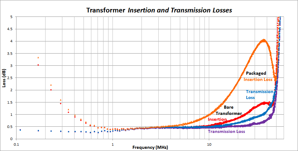
First, note that the transformer has low transmission loss up to nearly 50MHz. However, the insertion loss of the packaged transformer would be intolerable on the 10 meter band if it appeared the same way with an antenna wire connected.
Driving the End-Fed Wire
I strung up a nominal 80m half-wave antenna wire into the trees, snaking it through the open screen door to the work bench where I was doing the tests. Not the ideal antenna, but convenient! Connected to the packaged transformer, I ran some SWR sweeps with just the bare wire and various configurations of small coils to act as band-tuning compensation. The overlaid VSWR plots are shown below.
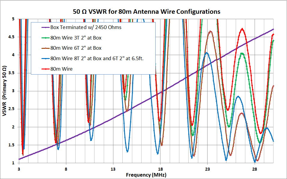
Just the bare 80m wire is shown in red. In the problematic upper bands, the resonant wire significantly improved the in-band SWR compared to the resistively terminate box (purple). I wanted to test the hypothesis that an inductance near the box would compensate for the output capacitance and further improve match on those bands. I place a 2 inch coil of the antenna wire with 3 turns (green) or 6 turns (brown) close to the box. The in-band SWR improved significantly with this localized inductance to compensate for the box’s capacitance.
The wire as I strung it up seemed to resist having a good SWR for the 20m band. There could be any number of reasons for that, where I put the bends in the wire, the location of tree branches, etc. It is common to use “compensation” coils of a few turns of the antenna wire to improve the alignment of the bands. I decided to play with this to see what I could accomplish. The blue trace above shows the results of adding a 6-turn 2″ coil about 6.5 ft. from the box. One interpretation is that this places the coil along the wire where there is becoming significant current in the upper bands and the inductor has more effect, compared to 40m and especially 80m where this location is near then end of the longer resonating length and where the current is almost zero.
It is very hard to know what will be the best solution for a given antenna installation if you want to hit all of the bands exactly. I suspect that a small coil near the transformer is generally a good idea, whether it is my transformer design or others, since it is very difficult to get the antenna wire out of the box without incurring some excess capacitance. The band compensating inductor placed on the wire is another story. How big and where to place it is likely best determined empirically. I came up with a very simple way to build these coils on the antenna wire that proved quick and easy to change and test, involving small piece of PVC pipe and a piece of Velcro shown below.
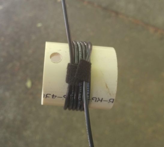
With tension on the antenna wire, you can just roll the coil up/down the wire to try different positions as you are optimizing for a particular band. There is no substitute for playing with the analyzer, trimming the wire, adjusting the compensation coils, etc., and going through the process for a few iterations to get the multiband antenna to work well for you as you have it installed.
Packaging and Thermal Performance
As is often the case, packaging was determined by what boxes I had laying around. However, I think I made a good choice with a Hammond 1590A diecast aluminum box. I installed an eyebolt on one end as a pull-point, and a BNC connector on the other. I fashioned an antenna connector with washers made from some acrylic rod I had on hand. The transformer fits sideways in the box with a few millimeters to spare. One point of my small-core, compact winding design was to be able to cool the core. The aluminum box is the logical heatsink, so I cut a few scraps of aluminum to make a thermal connection to the bottom of the box and to the lid, adjusting with aluminum shims so that when the box lid is screw down, the entire thermal assembly, with the cores in the middle, is under a little compression. If you really wanted to push this design, you could include thermal grease or thermal pads in the stack-up to improve the heat transfer, but I chose to keep it clean and see how it would do without any special effort.

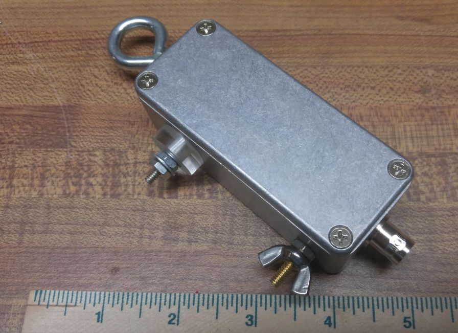
In the open-box image above you can see the thermal probe I used to measure the ferrite core temperature for a thermal characterizations.
The goal of the temperature characterization is to determine how much temperature difference (core to ambient) there will be for a given level of power dissipation. To this end, I weighed the main components of the box and looked up the specific heat capacities to get an approximate overall heat capacity for the entire box.
| Material | Mass | Specific Heat (J/g/C°) | Heat Capacity (J/ C°) |
| Aluminum | 130 g | 0.897 | 116.6 |
| Ferrite cores | 28 g | 0.8 | 22.4 |
| Steel (eye bolt) | 23 g | 0.45 | 10.4 |
| Total | 181 g | 149.4 |
Newton’s Law of Cooling tells us that heat flow is proportional to the temperature difference. The cooling rate is more difficult to calculate because it involves how heat moves through the structure, but it is easy to measure. I placed the box in a cool oven and let it get up to about 200 °F, soak for a while, and then I took it out, hung it in still air and measured the temperature as time passed and the box cooled. The cooling curve I measured is shown below.
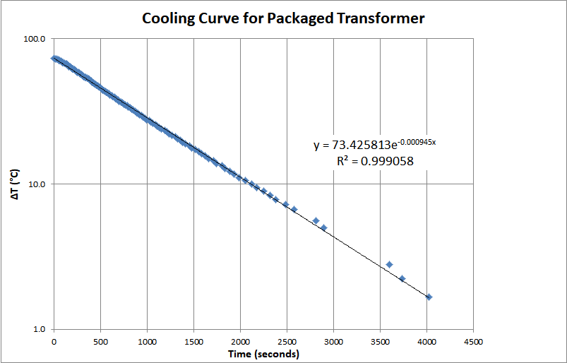
Graphed with a log scale, it makes a nice straight line. The point is to get the characteristic time constant for the cooling, which is the reciprocal of the exponent coefficient that Excel shows for the fitting equation. In this case τ=1058 seconds, about 18 minutes, is the characteristic thermal equilibration time in still air. It is hard to wait an infinitely long time for the box to equilibrate to a given power level. It is much easier to wait ~2τ, know that you are going to see about 86% of the temperature change you would see if you waited until time infinity, and just make a simple correction. At equilibrium, the heat leaving the box due to cooling will exactly equal the heating power input. The change in heat content in the box as it cools can be written:

where 


which gives the power dissipation simply in terms of the heat capacity, cooling time constant and the temperature difference from ambient.
With the cooling curve and a good estimate for the heat capacity of the box, now it is just a matter of running some power through the transformer and measuring the the temperature rise from ambient to be able to determine the power that turns to heat in the transformer. I chose to use FT8 transmissions for this test since they generate 100% duty cycle during the transmission period with an average duty cycle of 12.6 sec / 30 sec = 42% overall when including the listening periods. I found that sometimes the multimeter that was measuring the temperature would give unreliable information when RF was present, so the off periods provided regular intervals for measuring the temperature. The procedure was to run for around 30 minutes starting from the box cool at ambient temperature. Then record the change in temperature recorded at the core from the probe, and the elapsed time so I could corrected for not reaching perfect equilibrium. The results are presented below.
| Band | TX Power Level (W) | Average Power (W) | Time (min) | ΔF° | ΔC° equ | Pdisp (W) | η (%) | Loss (dB) |
| 80 meter | 50 | 21 | 30 | 21 | 14.2 | 2.0 | 90.5 | 0.43 |
| 40 meter | 50 | 21 | 30 | 16 | 10.8 | 1.53 | 92.7 | 0.33 |
| 20 meter | 50 | 21 | 33 | 15 | 9.8 | 1.39 | 93.4 | 0.30 |
| 10 meter | 50 | 21 | 33 | 16 | 10.5 | 1.49 | 92.9 | 0.32 |
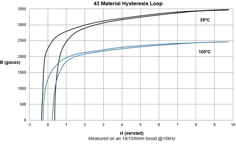
The biggest uncertainty in these measurements was the actual power level used. I used my IC-751A’s power meter and an in-line Siliconix power meter as well as a voltage probe on the feed cable. The SWR was low, but not unity, so the peak voltage was lower than the 50 ohm match value when measured with the high-Z scope probe. Typically the IC-751A would read about 60W on its power bridge, the Siliconix would show >50W on the 50W scale and 45W on the 500W scale, so there is ~20% uncertainty. These four data points are plotted on the Transmission Losses chart shown below as the yellow squares, all but the 80 meter point coming in a bit lower than expected losses based on the VNA measurements. One possible explanation is that the core losses drop with temperature. Note the material 43 hysteresis curves shown below for 25 C and 100 C has a smaller open area (and hence lower losses) at the higher temperature. I thought to test this hypothesis by measuring the losses as an oven-heated transformer box cools down. The results are shown below.
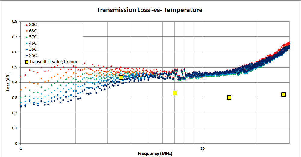
Below about 7 MHz, transmission losses increase as the core temperature increases. Above 7MHz, there is very little temperature dependence at all. So the differences I see in the data sheet’s hysteresis curves are not the correct explanation. Nevertheless, this is a rather curious result that might have derating implications for the 160 and 80 meter bands.
Maximum Flux Levels and Power Scaling
Scaling the small core to higher power levels would mean that the flux level in the ferrite core would increase. The maximum B field in the core is proportional to the imposed voltage, 

where A is the cross sectional area of the core, f is the frequency and N is the number of turns. For our transformer at 100W (==> 71 Vrms into 50 Ω ) , the core cross section for the two FT114’s is 0.74 cm2 , consider the lowest frequency as 3.5 MHz and our 5-turn primary, then plugging in the numbers we find Bmax = 0.012 T. Lets consider a much more challenging extreme: 1000W and the 160m band. Then we find Bmax = 0.076 T.
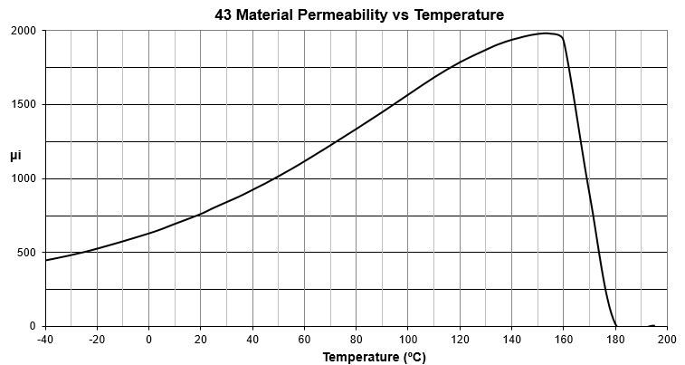
The Type 43 data sheets show us what we have to look out for. Saturation of a warm core happens near 0.2 T (2000 g) and if you don’t want to deal with significantly reduced permeability, then better to limit to 0.1T. The permeability rapidly goes away above the Curie temperature, about 160 °C on the data sheet. To be safe, better not get much above 120 °C.
Hence, even operating at 1000W on the 160m band, the cores would not saturate with the 5-turn primary.
The real power limit will be core heating. If we wish to limit the ferrite temperature to 130 °C, then assuming ambient temperature of 30 °C, we can tolerate a 100 °C temperature rise. From our measurements of the box cooling curve, this would correspond to the box dissipating about 14W in still air. Being conservative, assume we are just 90% efficient, then the average power level we could support would be about 140W. Or transmitting about 50% of the time, the peak power you would want to run with would be about 300W.
It is all about getting the heat out. Steps to improve the heat transfer over the present design could make this small transformer work at even higher power levels. Thermal gasketing between the cores and the aluminum heat sinks could help a lot, as would a single piece of aluminum rather than the stack up of thin sections I used. If you really want to get the heat out, add some fins to the aluminum box.
As you look to use this transformer at higher power levels, I can imagine that the bottleneck might be voltage breakdown or corona in the windings. I’m a hundred watt guy, so do not have a lot of experience with high voltage RF, but I know that ~5kV peak-to-peak RF voltage that you would expect at the 2450 Ω output at kilowatt power levels could begin to cause you some trouble.
End-Fed Wire NEC Model
I look at the end-fed as just an extreme example of an off-center-fed antenna. With very little counterpoise, the antenna is being fed at a high impedance point so a rather large impedance step-up is employed. To explore parameter space a little, I modeled a couple of lengths for the counterpoise and see how the wire is resonant across the band when fed with various impedances at the driven point.

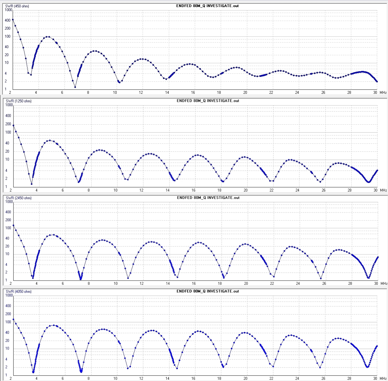
If you stare at the above frequency sweeps you will discover a few things.
- With a very short counterpoise it is difficult to resonate the fundamental with any drive impedance.
- Increasing the drive impedance tends to move the resonances to slightly higher frequencies.
- Adding an additional 2 meters to the counterpoise did very little to affect the resonant frequencies, much less than adding that length to the main wire would accomplish.
- The usual problems of having the multiple band resonances all line up appear here with the end-fed design, similar to the same issue with off-center-fed designs.
- “Best” results are with 2450Ω drive impedance and the 3.3m counterpoise, so it is not surprising that 49:1 transformers are the common choice.
Counterpoise
The model results show the need for a not entirely insignificant counterpoise. My limited experience with these antennas also suggest that one must be cognizant of the RF current pushed onto the feed-line coax. I set up an EFHW for field day using a similar transformer with 25 ft. of coax from the box, everything floating, to my battery powered radio. Transmitting on 15 meters was impossible because of RF into the radio. The solution was to make a small coil of the coax feed line, thrown on the ground, before connecting it to the radio. This gave the RF some place else to go, trapped by the coil and capacitively shunted to ground, rather than on to the transceiver.
Conclusions
Wideband RF components ultimately succumb to the non-ideal behavior of materials and assembly methods. In the case of the EFHW 49:1 transformer, the major shortcomings of the most popular current designs are excessive leakage inductance and poor heat transfer from the ferrite material to the environment. Tackling both of these issues at once led to a much smaller, lighter, and less costly transformer with better loss characteristics than previous designs.

Great article!!!
Renee KC3NG
Wow, Gary! Impressive article and so well done that I may give it a try. Above my old grey-haired head to be certain BUT well written enough to guide the neophyte through it all. Thank you for an interesting and informative read.
Thank you Gary. Most informative and appreciated. Frank VK1VK
Very interesting design. I made one quite similar to it but 3T Primary with #16 speaker wire (2 parallel wires) and 15T Secondary close wound just using about one-third of the circumference of the 2 inch toroid. It tests out well on the antenna analyzer for 3.5 to 29.7 MHz. Regards VE9HAM.
Gary, bravo sir! Wonderful experiment on a complicated subject. Thank you for taking the time to share your findings.
73 DE KN6UIZ
I love the science here. I’ve been trying to gain a deeper understanding of these magical transformers for years.
I’m curious that you used a 1:36 (5:30 turns ratio) transformation here. any particular reason?
Hi Charles, The transformer is wound as an autotransformer so the total turns of the secondary is the 30 + 5 of the primary, the primary just gets 5, so 35:5 is 7:1 turns which is 49:1 impedance. If you look toward the end of the article you will see the NEC plots for various drive impedance. I like the looks of 2450 ohms best which is 49 X 50. There may be cases where something else works better, but 49:1 seems a pretty good compromise.
Gary, thanks for sharing your experience with this stuff. I too wind my resonant EFHW antenna transformers autotransformer style. It never made sense to me how most wind them including the twisted pair at the primary section. To me, I think of the autotransformer as providing taps where you select the desired impedance appropriately.
One question: why is everyone using #43 material when it’s deemed by various sources as a less than ideal transformer material at HF frequencies. I guess that it is good for providing high impedance in common mode chokes. I read something K9YC wrote saying that #67 is a better material for HF transformers up to 50 MHz.
I rely on #43 toroids for choking RFI sources in the home and used to use it for EFHW transformers but recently started playing with #67 for end fed transformers. So far the empirical results are very encouraging and I plan on diving deeper into making measurements and getting to the facts when time permits, perhaps this winter into spring.
Ref: perhaps read the second half of p.29, here, and ponder: http://www.audiosystemsgroup.com/RFI-Ham.pdf
Paul, Great question. If I had other material on hand, I would have tried it! If you look at my other post on Performance of 49:1 transformers, I did compare a core materials I had on hand. No question that type 43 is going south as you approach 30 MHz. I had a “mystery” core with lower permeability that was still working at 30MHz which might have been one of these other mixes. So yes, I think that is a good idea. The down side will be lower permeability so more turns and a little harder to control leakage inductance.
Will stacking two FT140-43 handle 100W in 49:1 configuration easier?
Sure… but leakage inductance will go up because of the larger area so perhaps the 10 meter end will suffer… its all a compromise! Test test test!
I dare ask . You’re so far above my knowledge base. I read this because I have seen the Farrite saturation occurs due to heat. My question is how does the heat sink not affect the Farrite function?
Actually ferrite saturation happens when all of the little magnetic domains are pointing in the same direction and they can’t be any “more magnetized” than they already are. Relatively suddenly the change in magnetic field as the current is applied goes to the free space value – dB/dt that is the voltage opposing the rise in currents get very small, the inductance gets very small… That’s saturation. Heating can come about from a couple of things. First, cranking those little magnetic domains back and forth costs some energy ( and leads to an open hysteresis loop). Secondly, if the core material is at all conductive, you can drive currents in the core that will generate resistive losses.
As to the heatsinks — with a torroid, most of the magnetic flux wants to be in the magnetic ferrite material, which is a closed circuit with a torroid. The aluminum heat sinks are not magnetic, so the magnetic field pretty much ignores its presence.