The Off-Center-Fed Dipole Antenna – Design

There are a few ways to build multi-band HF antennas.  These include multiple resonant dipole arrays, trapped dipoles, resonant loops and the off-center fed dipole, OCFD.  I’m going to look at the OCFD because it is relatively simple to construct, yet gets quite decent performance.  I also am fortunate to have some nice tall trees from which to hang such an antenna.

OCFD Pros:

• Simple construction
• Multi-band operation
• Horizontal polarization
• Low radiation angle with good efficiency
• Has preferred propagation direction which can be aimed

OCFD Cons:

• Usually requires an antenna tuner
• Usually requires a matching balun
• Has lobes and nulls which may limit coverage to some areas
• Is not a beam

The ham bands are laid out across the radio spectrum at rational frequency multiples of each other – more or less.  This wise decision, made many years ago, allows relative ease at using the same piece of wire to receive more than one HF band.

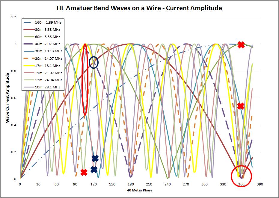
The chart above plots the standing wave amplitude of waves on a wire that all start with zero amplitude on the left side.  If you cut the wire where you again have an amplitude zero, a standing wave would be supported on the wire.  Arbitrarily, I chose to express length as the phase on a 40m long wire.  Note that many of the bands are close to resonant at the 360° (40m) point.  The exceptions are the red crosses at 360°, namely the 160m, 60m, and 30m bands.  An antenna made this long will completely fail with the 160m and 60m bands, and will have some difficulty on 30m.  In fact, 30m is problematic in general because the actual ham band is not a very close multiple of the others, so will often require more of a compromise.  The lowest resonant band on the 40m wire is the 80m band, hence a wire this long is classified as an 80m dipole.  If you didn’t have enough space for the 80m antenna, you could consider stopping at the 180°  point on the chart, where again there is another convergence of zero amplitudes for the 40, 20, 15, and 10 meter bands; or maybe you could stop at 250°  and attempt to capture the 60, 15, 30, and 12 meter bands.  Picking the zero convergence selects the overall length of the wire, but we still have to pick the dividing point where we drive it.

There is a nice design that picks the point at 120° as the driven point (the small black circle on the plot).  The 80, 40, 20, 17, 12, and 10 meter bands all have roughly the same amplitude at this phase along the wire.  This means that they can all be driven with a similar amount of effort from the transmission line (about the same impedance for all bands).  There are two bands that are not driven very well at this point, the 30m and 15m bands (black x in figure).  A commercial antenna system, the Buckmaster 7-band OCF Dipole, exploits this property.  The big advantage of this design is that you can make an antenna that does not require an antenna tuner by utilizing the constant impedance of the happy convergence that happens at 120 degrees.

I didn’t go for that design, however, because I really want the 15m and 30m bands as well.  I felt that both of these bands are more important than the 12m band, which is poorly driven with my design.  I picked about 103°  along the 40m wire as the operating point for the feed.  The red oval shows the wave amplitudes for the various bands at my chosen feed point.  There is quite a range over which I need to drive the antenna.  Hence we will likely find that it is not possible to get a fixed impedance for all bands, but will instead need to provide an antenna tuner to aid with the matching.  At this point I broke out the computer simulations for fine-tuning the lengths, to see what the radiations pattens should look like, and to get a better idea of how I would have to drive the antenna.

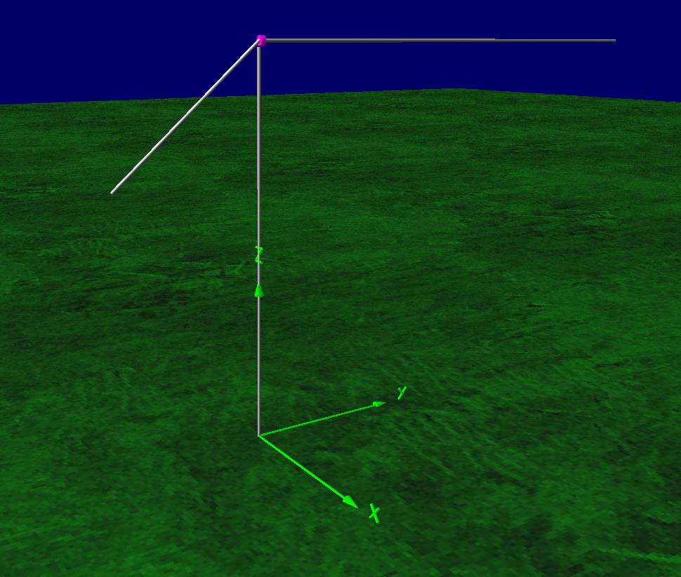
I had tall support points in the trees for the feed point and the far end of the long wire.  The short wire would be pulled down to a lower fastening point.  The model, shown in the figure on the right, includes the feed coax.  The feed is not connected to either main element since a balun is used to drive the dipole.  However, it is an easy matter to connect the vertical feed line to one side or the other and add a choke somewhere on the feed to get yet more interesting resonances.  Such tricks are employed with “Carolina Windom” antennas.  My model runs suggests only minimal changes if you connect up a vertical element so we will not further consider this modification here.  As-is, the vertical cable run is not particularly resonant with any band and has little effect whether it is included or not.

Specifications for the AF7NX OCFD:

Long leg:  93′  #14 THHN copper wire.

Short Leg: 37′ #14 THHN copper wire.

Height of feed point:  75′

Angle of short leg:  40° from horizontal (flatter is better)

Feed:  4:1 Balun to 75 Ohm CATV cable to Tuner.

The figure below shows the antenna tuning plots. (Click on the plot to get the big picture.)

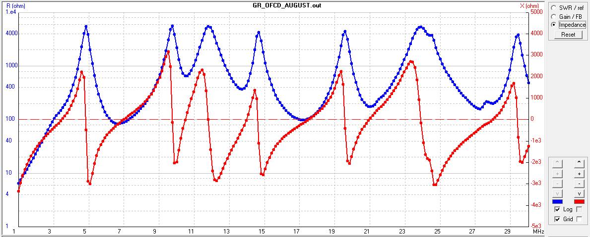
The antenna is at a resonance when the reactance term (red line) crosses zero.  Those points should be close to the ham bands a 3.5, 7, 10.1, 14, 18.1, 21, 24, and 28 MHz.  Most resonant frequencies are close to the desired ones except for 24 MHz (12 meters) which we knew was not going to be possible.  At the resonances, the resistive term will be the antenna driving impedance.  There is quite a range over which the driving impedance varies, from ~90 Ω at 7 MHz to ~700 Ω at 10.1 MHz.  The best we can to is select something in between 90 and 700 ohms.  With my 75 Ω  co-ax using a 4:1 balun brings the impedance of the driver to about 300 ohms, which is a good compromise.

You can see the band resonances on the SWR-300 Ω plot.  Portions of the 80m, 20m, 15m, and 10m bands could be used without a tuner if you have a 75 Ω transmitter, but our plan is to match with an antenna tuner at the transmitter anyway.  The antenna tuner will ensure that reflected power returning from the antenna will not be sent along to the 50 Ω transmitter.  Hence, any power reflected from the antenna must be re-reflected back to the antenna again at the tuner.  If there were no resistive losses in the feed components, we wouldn’t care at all about the SWR, since eventually all of the power would be radiated from the antenna after several bounces back and forth to the tuner.  But there are fintie losses in the cable, so too many reflections will sap transmitter power.  A good discussion of line losses and SWR can be found in this 2006 QST article. The numbers in the brown shaded column in the table below come are derived from a graph in that article. The table also shows some of the numbers from the NEC model runs (shaded blue) for each ham band.

 

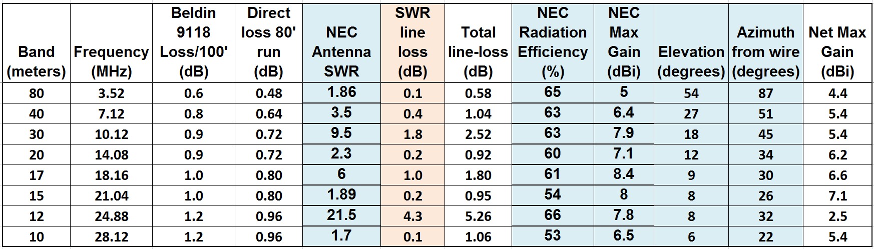
For our 80 foot run of Belden 9118 coax, the overall transmission efficiency is respectable for all but the 12m band, where we expected problems; even so, 12m is marginally useable. The 30m band is also a little less well-coupled than one might hope, but this is a particularly difficult band to get to resonate well with the other frequencies on the wire; 17m has the same problem to a lesser extent.

It is worth pausing to consider the effects of the SWR mismatch on both the transmit and receive operation of the antenna.  It doesn’t matter which way the signals are going, there will be losses associated with the SWR in the transmission line, but the overall effect on performance is quite different in the two cases.  On reception, the critical figure of merit is the signal to noise ratio at the receiver and NOT the total signal level.  Almost always, the limit to noise performance is “atmospheric” band noise and not the noise limit of the receiver.  Lets consider the 12m band where we have 5.3dB of line loss, mostly associated with SWR from the poor match.  If we are listening to a transmitter coming toward one of the high-gain lobes of the antenna, we can expect that the signals on the antenna will be ~7.8 dB larger than the noise compared to what would come from an isotropic antenna.  On the way to the receiver we will lose 5.3dB, but atmospheric noise received by the antenna will also be attenuated  by the same amount.  If the receiver has enough clean gain to make up for this loss, we might be quite happy with the antenna performance during reception.  On transmit, however, all we care about is the relative amount of power aimed at our target receiver.  The 5.3dB line loss means that less than a third of the power from the transmitter will ever get out; two-thirds turned into heat in the transmission line.  If you normally run your digital mode at 15W now you will have to use 45W.  Of coarse, the antenna gain pattern still matters to be able to throw the power where you want it.

The table lists the maximum antenna gain for the low-elevation lobes.  Let us look at the radiation patterns that NEC2 gives us. Plots are the elevation and horizontal patterns for six of the bands supported on the antenna.

 

 

 

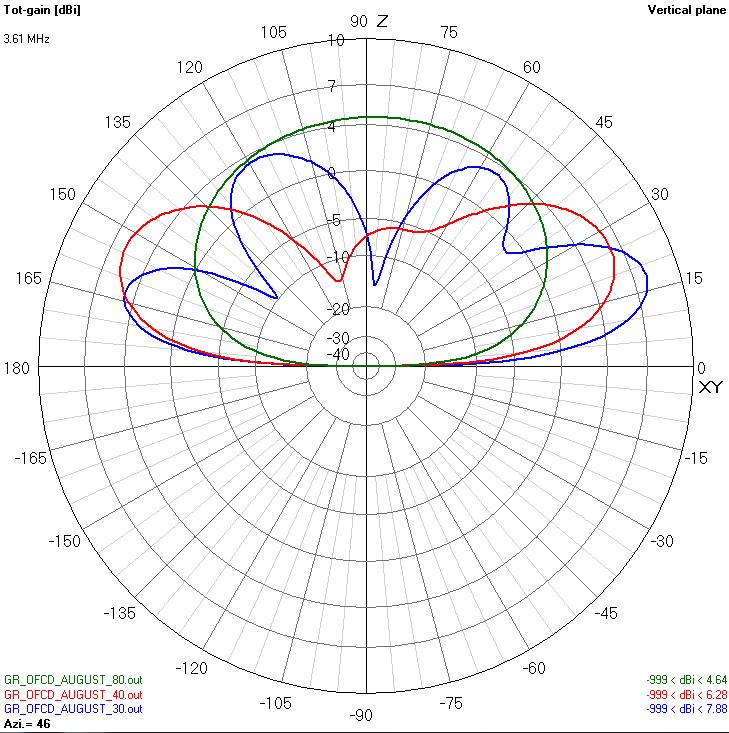
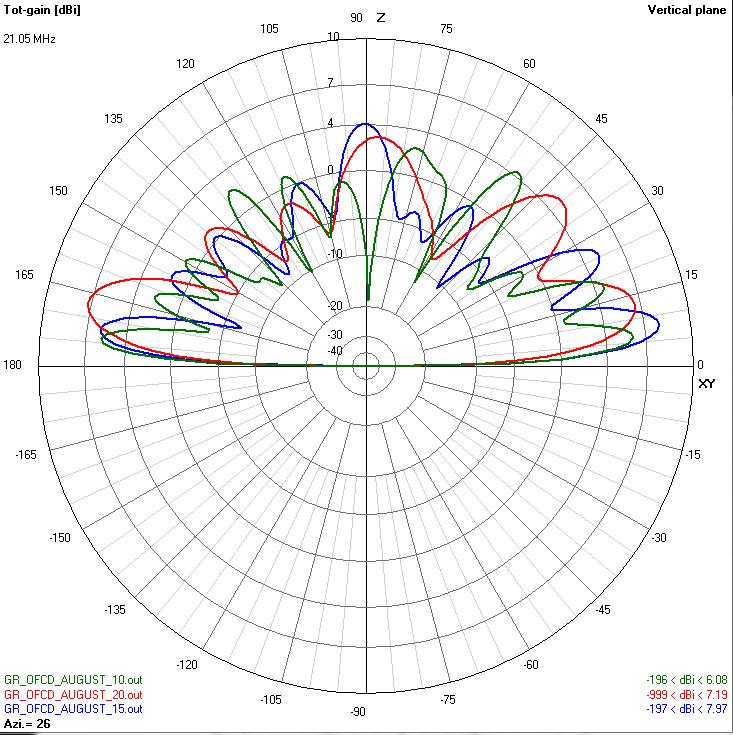
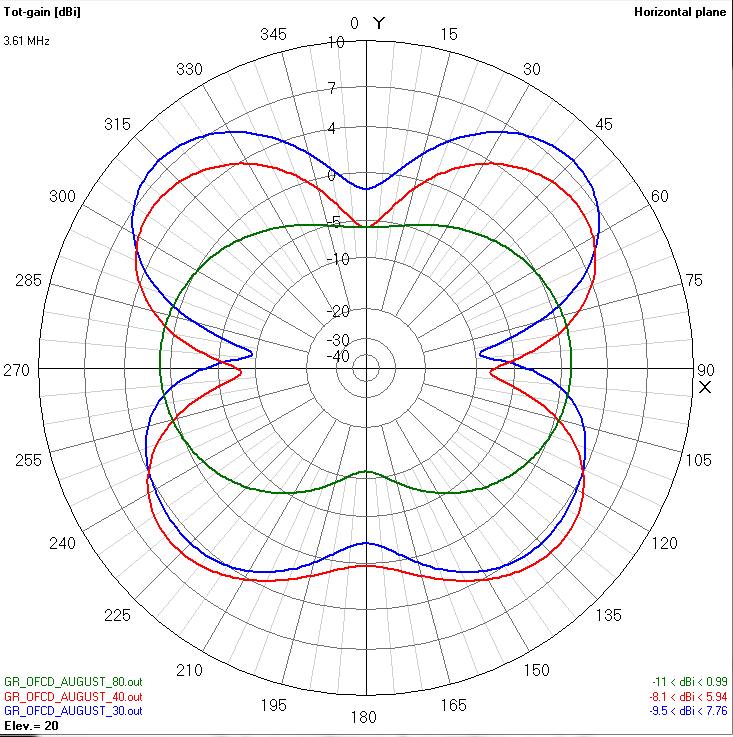
Notice the progressively lower maximum elevation peak as you progress to the higher frequency bands.  Looking at the horizontal pattern notice the low gain off of the end of the antenna in the Y direction.  Also note that the maximum for the radiation pattern is not strictly broadside to the antenna except for the lowest fundamental 80m band.  For the higher bands the largest lobe swings around to pointing 50 to 20 degrees from the antenna wire, depending on the band.   I’ve aimed the antenna so that Europe is about 35 degrees from the direction the wire is pointing to attempt to take advantage of one of the high-gain lobes.

Finally, one last pretty picture of the propagation “rose” for the 20m band.  The pattern is complicated with multiple lobes at several elevations.  The nice strong low elevation lobes are quite narrow and oddly spaced so it is hard to know exactly what the antenna is actually pointing at.  The strongest stations you hear might just happen to be lined up to the pattern, and you might miss stations seemingly close by that are just outside the best directions.  This antenna just adds a little more contingency to the already very contingent whims of propagation, but it is simple and surprisingly effective.

I’ve got this antenna up in the air now.  It works pretty well. In a future post we will look more carefully at its actual performance.