Comparing Receivers with Digital Mode Signals

I entered second heaven when I got my second radio.  My original 32-year-old Icom IC-745 got placed on the back shelf when the new 29-year-old Icom IC-751A arrived.  As much as I enjoyed the old IC-745, I was after a little computer control, and the 745 predates the idea that people use computers.  The 751A, just a few years later at the dawn of the PC age, at least had an optional serial computer interface.

Once I had two radios I could not help but to start to make comparisons.  Both radios do an admirable job, but I began to notice some small differences in the way they would handle strong narrow-band digital signals.  When I used the IC-745, I would turn the AGC off and manually set the RF gain so that I was just picking weak signals out of the static noise floor.  This meant that strong signals would be over saturated, but the 745 didn’t mind that too much.  When I tried to use the IC-751A the same way, the strong signals would generate signficant amounts of in-band spurious interference, mostly third-order intermodulation products (IMD3).

What happens if you don’t have your levels set right?  Most hams know that if you overdrive PSK signals during transmission, there can be IMD3 spurious emissions that can disrupt the band.  This appears on PSK signals as multiple “railroad tracks” that spreads out over the band.  Less well-known are the effects that come from improper receiver level adjustments.  The tricky part is that we need to process a very large dynamic range of input signals, all right next to one another.  The IMD3 problem shows up on receive as well as on transmit.  Here the problem is the mixing of harmonics of two in-band signals, where the mixing products appear back in the pass band.  The “third order” products are generated by the mixing of the fundamental frequency one signal with a second-harmonic of the second and vise versa.  With frequencies A & B, the in-band mixing products will be 2A-B and 2B-A.  If A-B =  Δ, then you will find spurs at A+ Δ and B – Δ.

The picture above shows a clear example of receiver IMD3 distortion.  The IC-751A had the AGC turned off so when the strong signal in the center of the waterfall began broadcasting, the front-end stages of the receiver were overdriven.  The same signals in the IC-745, with the AGC on, don’t have the problem.  Note the strong “mirror” effect of spurs across the strong signal.  If you were operating this way, you may be tempted to latch onto one of the traces on the right side ( above the IC-751A label in the figure).  The nature of PSK is that these spurs are decodable, but if you try broadcasting there, the sender will not be waiting for you.

Before we move on to the measurements, lets look at another set of spurs that have a completely different origin.

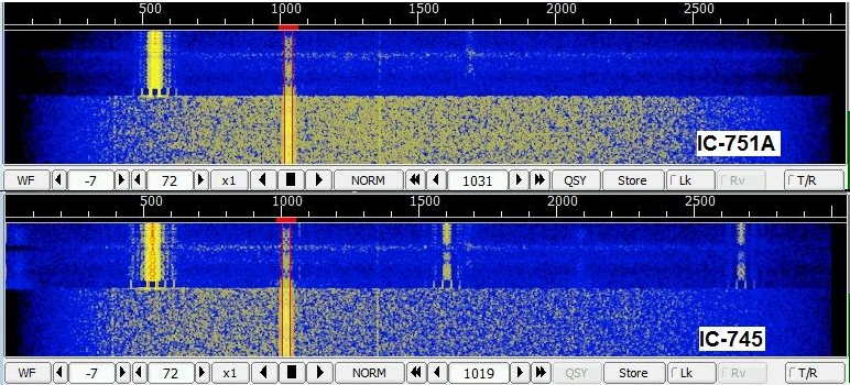
Note the two spurs at 1600 and 2680 Hz on the IC-745 waterfall above.  There is another strong signal in the picture, but the spurs don’t appear related to the frequency difference between them.  In this case we are looking at audio harmonics, the third and fifth, of the audio signal at about 550 Hz.  The odd harmonics will appear in the audio if you start clipping it.  In this case, the problem was that the sound card was being driven too hard on that strong signal.  The solution was simply to reduce the input level to the sound card.

It took me a while to realize that the IC-751A had significantly more RF gain than the IC-745.  If I set the manual RF gain on the 751A at about 60% of full, I had similar gain to the IC-745 at full.  But before I figured all of this out, I thought that the IC-745 had better noise performance the IC-751A.  But how to know for sure?

My test consists of splitting the antenna signal with a 50 Ω power tee so that each receiver gets the same signals from my antenna.  Then I set up both receivers to have almost identical noise characteristics on the FLDIGI waterfall.  I run two copies of both FLDIGI and  WSJT-X during the comparison.  Running WSJT-X, I set the input levels to have about 30 dB noise level between transmissions on both receivers.  This gives the decoders plenty of dynamic range and again matches the overall gain of both receivers for the digitized signals.   Now we just listen for a while and accumulate JT65 and JT9 signal reception reports from both receivers.  If everything is identical, you should get identical signal-to-noise reports on both rigs.  Comparing the two waterfalls can show where there are problems with one rig or the other.

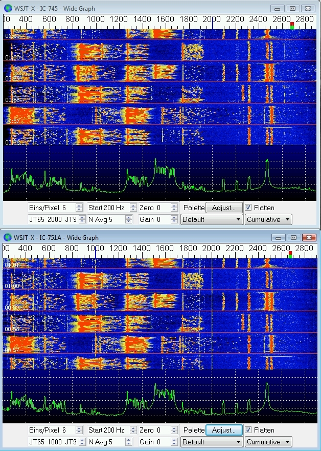
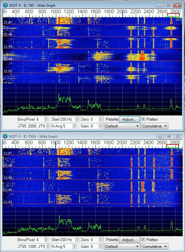
The JT65 and JT9 signals on a busy Saturday afternoon shown in the waterfalls above illustrate the dilemma.  Many of the transmissions are very strong, and weak signals may be intimately interspersed among the strong signals.  I found that I could get significantly better noise performance on a crowded band by reducing the RF gain below the point that the AGC would normally operate, especially on the 751A.  The waterfalls above were recorded with only 40% of max RF gain on the 751A and 75% of max gain on the 745.  Under these conditions, the signal reports back from the WSJT-X program are virtually identical between the two radios.  Both of my receivers can be made to show strong IMD3 spurs if the front end gain is allowed to get too high.  The AGC helps in this regards, especially with the IC-751A because this receiver has quite a bit more gain head-room in the RF amplifier than the IC-745.  Under extreme conditions manually turning the RF gain down even further seems to help.  JT65 signals can become a speckled smear across the band when there is IMD3 distortion from multiple strong signals.

In the midst of this exercise, my neighbor three blocks aways started calling on the PSK band just below the JT band in frequency.  This caused some trouble for the IC-745.  My neighbor’s +60 dB over S9 signals, only 6 kHz away from where I was tuned, made a mess of the strong JT signals.  I found it curious that the problem was greatest with the strong signals.  Clearly this is one place where the IC-751A had superior performance.

Measuring accurately the comparative noise performance of the two radios required analysis of the reception logs created by the WSJT-X programs.  The reporting on JT65 signals is compress at the high-end, the program never sending more than -1 dB signal level report.   JT9 on the other hand, robustly covers signal-to-noise levels from +15 dB to -28 dB.  This makes the JT9 signals much better beacons for our tests, however there tend to be more JT65 signals to be received.  I looked at both modes, but for JT65 I don’t consider strong signal reports larger than -5 dB in the receiver comparisons.  In short order it is possible to collect several hundred report pairs that can be used to get good statistics.  You can use my RX_compare spread sheet as a template to do something similar if you wish.

It is not too surprising that my two radios have essentially equivalent noise performance.  They were both considered “hot” receivers during their day. I would be really curious to repeat this little test, comparing a modern direct conversion SDR receiver with the classic superhetrodyne architecture my receivers have. That might show some real differences because of better IMD3 suppression in radios without so many mixers.

Now that I am convinced I can adjust the two receivers to accurately reflect the antenna noise performance without introducing their own bias, I can proceed to compare my two antennas.  Stay tuned!