Modeling the J-Pole

When you first meet the J-Pole, you are forgiven if you don’t quite grok how it is supposed to work.  What is that ‘J’ for anyhow?  When I have questions like this, I get out the 4NEC2 modeling program, and see what it says.  Let’s start out with the basic model — the J consisting of a λ/2 radiating section above a λ/4 “matching” section with the feed point across the ‘J’ near the bottom as shown in the figure to the right.  The J-pole is a monoband antenna so I developed a simple NEC model that has just a couple of parameters that allow for optimization for a given design frequency. 
Running the model and looking at the current distribution immediately illuminates how the antenna radiates. Currents are roughly balanced on the two parallel lines of the J as shown in the figure on the left. Hence, there is little far-field radiation coming from the bottom section, but the top half-wave section will radiate just like a vertical dipole.

Less obvious is how the matching works, but we can hazard some guesses.  The source is injected near the bottom of the J. The downward going wave quickly reaches the shorted end at the bottom of the J and is reflected back up.  There is a natural impedance transformation from near the bottom of the J where currents are high near the feed point, to the top of the J where the λ/4 line ends in an open circuit and where the λ/2 section is near its current minimum.  For power to flow out of the λ/2 section as radiated power, it first has to get into that section via the single-ended connection at the top of the λ/4 section.  The currents must be unbalanced at the top of the λ/4 section and the impedance must be finite to allow power flow into the λ/2 section.  This necessary unbalance is achieved by the superposition of the reflected downward and the direct upward component waves from the feed point.

The wave impedance at the point where current must flow up into the λ/2 section will be determined by the where and are the inductance and capacitance per unit length of the conductor at that point.  For a “single wire line”, calculating those values is a bit uncertain because you need to know where the E and B fields become deminimus and you have to do some complicated integrals in three dimensional space, but suffice to note that the conductor diameter matters the most.  Fat conductors have more capacitance and less inductance and hence a lower impedance than skinny ones.

For the sake of curiosity, I looked at how the feed point shifted and the amount of common mode feedline current changed as a function of the diameter of the radiating element.  I first optimized both the feed point location and the λ/4 section conductor spacing for the case of a 2mm diameter radiator.  Then I changed just the radiator diameter and re-optimized just the feed point location for best SWR.  The program lets you measure currents on the elements, so I recorded the current magnitude of the λ/2 section at its maximum in the center, and also current the heading down the mast where it connects to the J-pole.  The results are presented below.

Diameter of Dipole Section Element (mm)	Feed Point Distance from Bottom of J (wavelength fraction)	Optimized SWR from Model	Dipole Current Magnitude Maximum (A)	Common Mode Feed/Mast Current (A)	Ratio Feed line to dipole current (%)
0.4	0.0141	1.08	1.07	0.23	21
1.0	0.0146	1.04	1.02	0.25	25
2.0	0.0152	1.00	0.97	0.29	30
6.0	0.0162	1.05	0.86	0.33	38
10.0	0.0167	1.06	0.79	0.35	44
20.0	0.0169	1.06	0.68	0.38	56

It is pretty clear that when the conductor is a small diameter, the impedance is relatively high.  The feed point does not need to be as far unbalanced to drive the dipole section and the currents on the feed line are significantly less than if you were to try and drive a very fat radiating element.

You can look at the distance from the end of shorted  λ/4 section (bottom of the J) to where the feed point needs to be to get good SWR as the amount of “unbalance” required to force the required current up in into the radiating section.

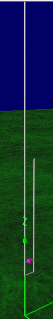
So far the model described above has neglected important real-world components — namely the feed line and/or conductive mast structure.  A more complete model is shown in the figure to the right.  The feed is separated into the “inside” of the coax with an ideal transmission line (blue) to the source.  The “outside” of the coax is modeled as an antenna element going to ground (it could be a conductive mast).  The J-pole has a modest common mode current that shows up in the model run.

As is often the case, Tom Rauch W8JI, makes some astute observations about the question of the moment.  He notes that the J-pole is basically just one more version of an end-fed design that runs into the “counterpoise” problem.  The current that needs to feed the λ/2 section has to come from somewhere.  The λ/4 section which looks like a balanced line must in fact not have balanced currents. Hence, to feed what looks like a balanced λ/4 line in a way that produces unbalanced currents must require an imbalance at the feed point, which implies that potentials will exist to drive currents down the mast or feed line coax.

The effect of the imbalance in the feed section can be seen in the radiation pattern, which appears not perfectly symmetrical.  But the feedline currents and pattern imbalance are small and in many circumstances can be ignored for the convenience of a very simple feed system.

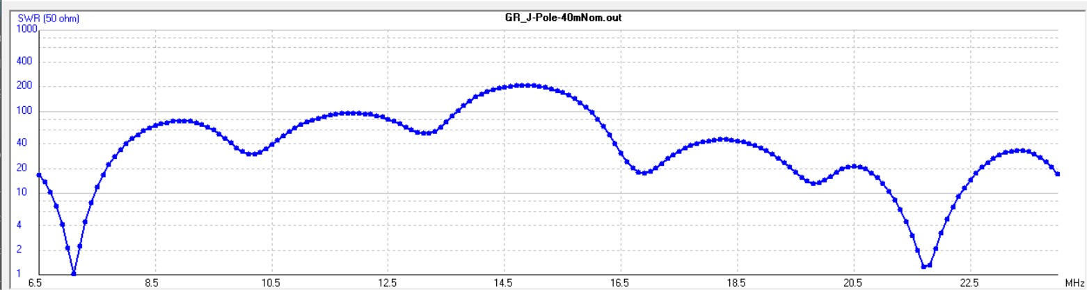
Since the J-pole uses a λ/4 matching section, chances are good that the matching scheme will work for any odd quarter wavelength, the next one being three times the frequency. Indeed, the model for a 40 meter J-pole shows a resonance on the 15 meter band.

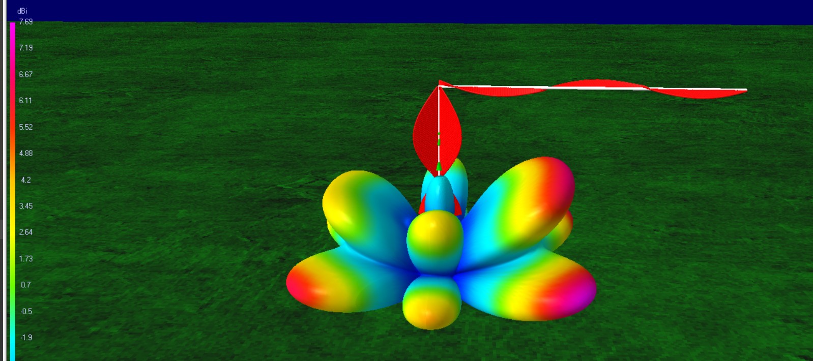
The problem with the third harmonic on a vertical is that the pattern is not very good. Most of the radiation is heading toward the stars with just a narrow near-horizon lobe.  How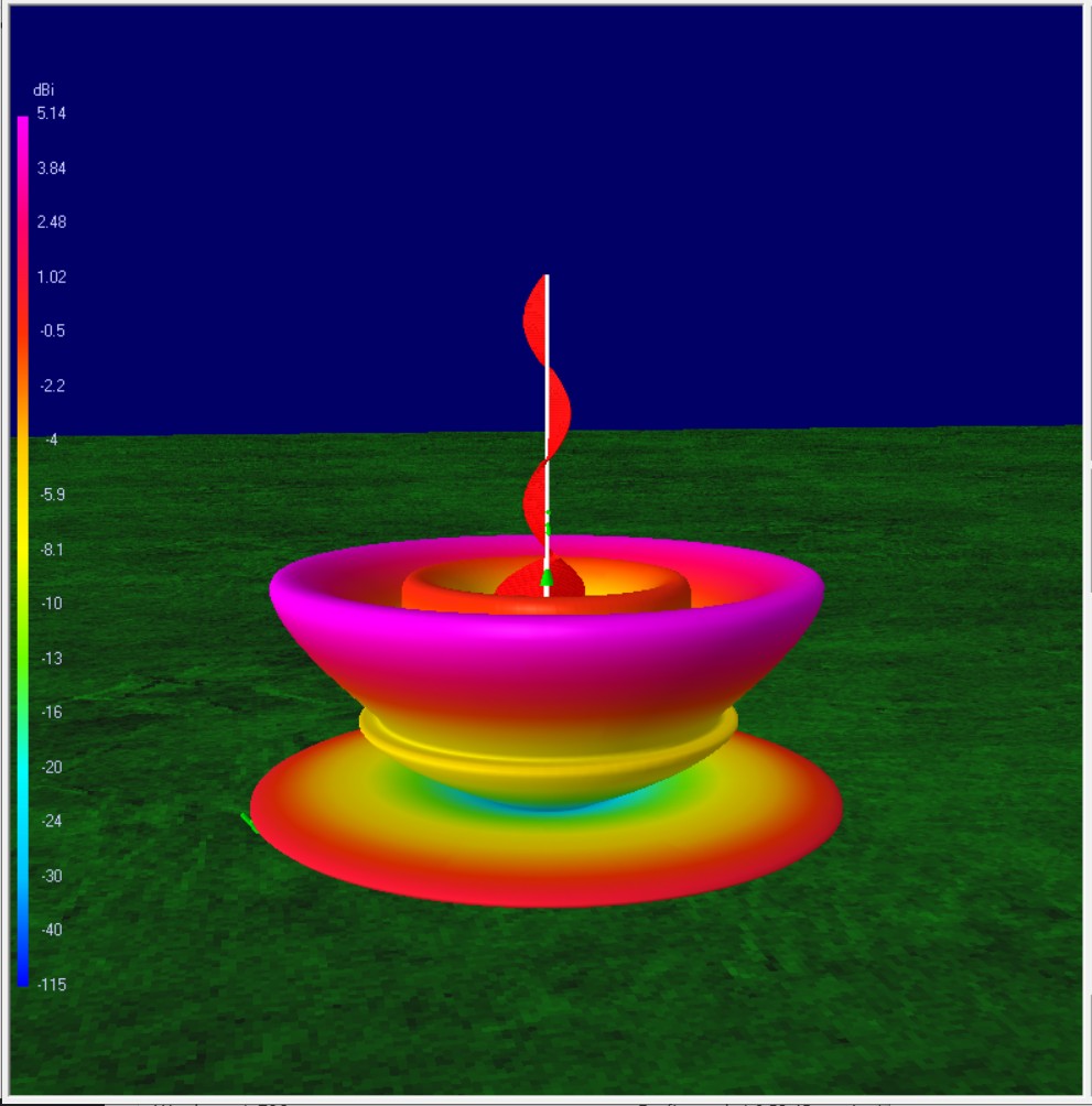ever there is nothing to say the J-pole has to be vertical.  The same scheme will work with whole thing horizontal, or with a kink between the matching section and the radiation section.  The third harmonic pattern is more useful with a horizontal antenna, as long as the lobes are pointed where you want to listen.

This last variant is commonly called the half-wave Zepp antenna, named after the Zeppelin dirigibles  where this antenna was commonly employed for communications.

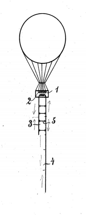
You can see the basic J-pole in this 1909 patent drawing  with the airship above the antenna hanging below the balloon’s basket.

The NEC model I used for these runs is listed here.  There are only two parameters to tweak to design a tuned antenna.  These are the position of the feed point tap, and the wire spacing of the λ/4 section (which determines the line impedance).  The feed point is the most important free parameter for a good match, but to get a near-perfect match you need to also adjust the impedance of the λ/4 section.

The J-pole and its cousins should be in the radio amateur’s tool box of tricks because it is an easy to deploy antenna.  But like other end-fed designs, you do need to be cognizant of feed line common mode currents.