
When it comes to understanding the performance of HF antenna systems, there are only a few tools. You can measure the impedance match with an antenna analyzer, you can model the antenna to see what you might expect the antenna to do, and you can listen and talk on the air to see how well you are heard. There are some weak signal modes like WSPR and the popular FT8 and their associated reporting networks that can tell you where you can hear and where you are heard, but the vagaries of propagation make any kind of quantitative assessment almost impossible. However, with the advent of the WSJT-X weak signal modes there is another way. Thanks to the signal processing in the WSJT-X software, the signal from every received station also gets it own signal-to-noise (SNR) report. The SNR report tells you the signal level compare to the background noise level that is being concurrently received by the antenna, which by itself may not be particularly illuminating. However, if you wish to quantitively compare two different antennas, then these signal reports from stations around the world are gold.
I described a way to measure the antenna pattern of a fixed wire a few years ago when the JT65 and JT9 protocols were widely used. The method involved Excel spread sheets, needed a lot of hand manipulation of the data and was laborious, but it worked. Fast forward a few years, and I still find myself needing a way to make these measurements, but I don’t want the labor overhead. So I decided this was the perfect project with which to learn the Python programming language and build a useful analysis tool at the same time; allplot was born.
allplot takes its name from the ALL.TXT files that the WSJT-X software generates in normal operation. The ALL.TXT file is a log of everything received and sent by the program. The reception reports include a time stamp, the station call sign, often a grid square locator, and the SNR report. A typical experiment involves collecting two simultaneous sets of reception reports, using two receivers, from two separate antennas that can then be compared. The allplot program accepts the two ALL.TXT files, finds all of the simultaneous transmissions received by both antennas, matches up grids and callsigns, looks at differences in the SNR reports and generates averages over grid square locations…and so on.
Main features and uses of allplot
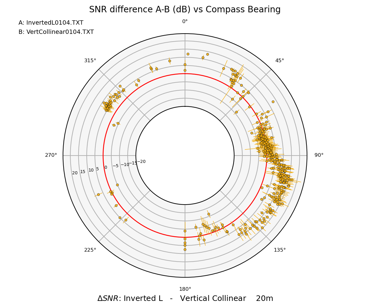
The best way to see what the program does is to look at some sample data from my antennas. Below I show some data collected from my Inverted-L big wire that is up in the trees about 100 ft. high, compared with my vertical collinear 20m antenna. The vertical is an axisymmetric antenna so there is little reason to think there is any directional preference coming from this antenna. The first thing we can do with the program is to look at all of the averaged SNR differences on a polar plot. The program also provides summary averages overall of the data by band.

| Band | SNR A-B (dB) | Stdev |
|---|---|---|
| 160m | 3.18 | 1.84 |
| 80m | 3.73 | 2.13 |
| 40m | 1.3 | 2.65 |
| 30m | 5.18 | 1.81 |
| 20m | 5.14 | 3.13 |
| 17m | 2.46 | 3.07 |
| 15m | 2.42 | 2.97 |
| 12m | 0.50 | 2.38 |
| 10m | 3.08 | 2.27 |
From the summary data we can see that the Inverted L is outperforming the Vertical by `~2 to 5 dB on almost all of the bands. This is not surprising for a high horizontal wire. The summary data will be skewed in favor of where most reception points are located, so should be considered only a very rough comparison.
More interesting is to drill down a little. Let us look just at the 80m band. (click on the images for a better view)


Besides the single band polar plot, allplot can generate a heat map of the reception signals based on their point of origin. We can identify the mass of red and orange points on the map in the eastern United States with the large cluster of points on the polar plot with bearing between 60 and 120 degrees. This is the “good lobe” for the Inverted L antenna. Regions to the south and north into Japan do less well, often with the vertical giving the best performance.
On upper bands, there are more lobes and nulls in the pattern off of the big wire. Look at the dramatic null into the northeastern USA for the inverted-L on the 20m band compared to the enhancement into Florida.

The polar plot and signal mapping are probably the most useful functions of allplot, but there are some fun things as well. The program can generate animated maps of the signal reception reports. (double click for full screen) This is similar to the PSK Reporter map, but animated, and you can see symbols for either or both antennas that hear the station. When both antennas hear a station, then you can map the SNR difference between them. That is what we see with the second animation below.
Sometimes you might wish to compare the propagation pattern of a single antenna under different conditions. For instance I was curious about the front to back characteristics of my hex beam so I made two data collection runs with the antenna turned 180 degrees on the second run, comparing on both runs with the inverted-L. Obviously you cannot make a direct comparison with simultaneously received signals, but using simultaneous signals with respect to a reference antenna allows much of the propagation-dependent variation to be removed from the measurement.


The images above show the comparisons for the hex beam with itself turned from 100°E to 280°W. Even though the reference antenna, the inverted L, has a very strong variation in response on the 20m band near 90°E, that variation is almost completely washed out when making grid-by-grid averaged comparisons for the two hex directions. There is more scatter in the data as you can tell from the width of the band of points on the polar graphs and the size of the error bars, but basic front-to-back directivity of the antenna clearly shows up.
My hex beam is a multi-band antenna with two element wires for 20m, 17m, 15m, and 12m. I also added a single bent dipole element for 30m on the top. I was surprised to discover that the 30m dipole fires “backwards” from the main antenna. Next time I’m after 4J3DJ on 30m in Azerbaijan I will pointing this antenna the other way!
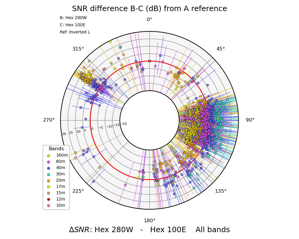

When you look at all of the bands on the polar plot, especially in the cluster of data toward the eastern USA, you can see the points for the upper band inside the red circle (favoring the antenna pointed 100°E); whereas the 30m aqua colored points are well outside the red circle (favoring the antenna pointed 280°W). The 40m and 80m bands, blue and purple points respectively, are not resonant on the hex beam so there is very little difference in reception when the antenna is reversed.
allplot Distribution
I was hoping to provide a compiled binary executable for the program, but so far that has eluded me. Python scripts can bury a tremendous amount of complexity in a few lines of code. That is certainly the case here. The script itself is only ~60kB of code text, whereas a compiled distribution folder is >1.3GB. I have been using the Nuitka Python compiler to try to build the compiled version, but I have been running into errors so for now that will have to wait. The script source and ancillary files are published on Github. The Python literati need only go there, pick up my script, and use it with their own Python installation, installing packages as needed. To install a complete Python environment on your computer that will run allplot, you can use the instructions linked here which are also included in the Github files.
Installing the Python environment in which to run allplot will take you about half and hour and consume ~4 GB of disk space. The program runs in a command window and generates in-line plots as you go along, or will save them to disk directly, as it does with the map animations. In the Python environment, you can edit the source code easily with a good text editor such as Notepad++ to make your own modifications and improvements.
Band Switching
Doing a few comparisons a single band at a time only requires setting up the two receivers and setting them to listen for a few hours. But a band at a time can be slow slogging if you want to fully characterize an antenna on all of the bands where it is useful. I looked around a bit for a good program to schedule band switches of the radio, but only found one that would do the job I wanted, namely HDSDR. If anyone knows of a better alternative I am all ears. HDSDR is a program designed to control and demodulate SDR receivers. I use it for the RTL-SDR I use as the pan-adapter for my IC-751A main HF radio. The program has the ability to control a radio connected via OmniRig to the HDSDR program, and can also control a program such as WSJT-X using the “CAT to HDSDR” connection. In fact, you needn’t even have an SDR radio to use the OmniRig and CAT to HDSDR features of the program, so the program will work with just about any radio.
HDSDR also has a feature to allow scheduled recording of broadcasts. I use this feature, but set the length of the recording to only 2 seconds to minimize the size of the WAV files created at every band switch event. Typically I set up a schedule that switches every two or three minutes to another FT8 frequency on another band. I use the same schedule, running two instances of HDSDR, to switch both radios in unison. This works well to monitor several active bands, with never more than about 10 minute silences on any band. A program to generate the band switch schedule, HDRSDR_Sked.py, and a couple of sample schedules are included in the distribution on Github.
Conclusions
When you have a new measurement tool you will discover new things you didn’t even think about before, and will likely generate more questions. I noticed on one overnight comparison of 160m antennas that the relative performance of the two changed during the course of the night, with one antenna better in the evening and the other better in the morning. What’s with that?! For radio amateurs serious about improving the antenna installations, allplot can provide quantitative guidance.

AFIK the report in FT8 and similar modes are not an indication of an absolute signal strength, as the ones we see in an S-meter. The ‘SNR report’ is an information, how strong a signal has been decoded compared in relation to other signals at the very same time in the audio passband. So, watching the same station, depending on other stronger or weaker signals in different FT8 cycles, may show complete different SNR values. Additional, comparing signals at two locations must come from exact same rig and absolute same settings in rig (AGC, filter, etc.) and the same settings in WSJT-X (bandwidth setting, input level, etc.). If all this is set, still unknown different antenna lobes of the two compared, may result in differences.
Part of what you say is true — part not. Indeed the SNR value given by the WSJT-X program is just a measure of the signal level compare to the entire band noise level. For this reason, I am only interested in differences in SNR reports on the same cycle coming from two different antennas. Under these conditions the “noise” conditions should be quite similar and also the instantaneous propagation conditions should also be quite similar. Hence the difference in SNR will largely reflect the antenna reception capability of the signal. The receiver characteristics can come into play in some cases, but usually not. Modern receivers have a noise floor significantly lower than band conditions most of the time. Best to run with the AGC off, but even if it is turned on, gain reduction will reduce both the signal and the noise level the same amount and not necessarily degrade or enhance the SNR report from WSJT-X. If there is a question as to the relative performance of two receivers, that too can be answered with allplot. You merely have to split the RX antenna signal and send it to both receivers and collect some data. If you see a systematic discrepancy between the two receivers, then you should do something about it before trying to use them to compare antennas. What I find is that quite disparate receivers tend to see pretty much the same thing in those type of experiments.
There are know situations that muck things up. If for instance, a single extremely loud signal can overload a receiver front end and distort or suppress the SNR reports from other stations during the reception interval. There is a “maximum SNR report” filter that will reject all signals from a reception period where any signal is found above the maximum threshold, which you can set. this effect can be receiver dependent, but in general I have not found it to be debilitating, and usually just leave this filter turned off.
I suggest you give it a try!
My understanding of WSJTX decoding and noise estimation is that is only depends on the information in the signal decoded and nothing else. A successful decode means that every bit transmitted is known and every bit received is known. The forward error correction will only allow correctly decoded signals through and then there is perfect knowledge of what was tranmitted.
The noise on the signal is the difference between known transmission and the actual received signal summed over all the bits of the transmission. This is then converted to equivalent SNR as if the signal was transmitted in an empty band with only thermal noise.
Other signals on the band may generate interference that add noise and degrades the SNR estimate.
The every transmitted bit known also enables the multipass decoding. The algorithm decodes all the signals it can, generates their know transmitted signals and subtracts that from the reception and runs the decoder again. It seems they do this several time in the more recent versions.
Yes, we have to give heaps of credit to Joe Taylor for inventing these modes and extracting all of the information that he does from weak signals. For the purposes of the allplot program, this is just black magic! What I have noticed (and is surprising to me) is that the SNR reported for signals that are covered by another transmission are very nearly the same when they are not covered. However, I have also noticed times when overdriven signals on the band result in a plethora of weaker signals getting the value of -24dB (too weak compared to reality) which must have something to do with the distortion due to the overdriven signals. Whatever the case may be, there is nothing like averaging thousands of observations to come closer to the truth!