
The simple 20 meter pull-up vertical antenna I described last time has been working well. I’ve been putting my efforts into working DX stations and have found that the vertical often does almost as well as the Off Center Fed Dipole (OCFD) despite its generally lower gain. Part of the reason is that there are places the OCFD does not hear very well, such as along its pointing direction, north into Russia. Also, the OCFD seems to do especially well to the east coast and southeast, and at times the band can be overwhelmed with signals that I am not interested in. With these effects taken together, the vertical dipole can sometimes offer better performance than the generally higher gain dipole.
Part of the motivation for the vertical antenna was so I could better map my OCFD antenna. When I tried to do that exercise comparing to my 40 m loop, there was too much uncertainty in both the loop model and the OCFD model to be able to make much sense of the results. However, comparisons with an inherently symmetric vertical antenna can directly generate the radiation pattern for the horizontal wire. So that was the plan; collect lots of JT65 and JT9 signals simultaneously on two receivers connected to the two antennas and make comparisons for lots of geographic locations.
Needless to say, it takes a certain amount of persistence to churn through the data collected over a week or two of leaving the radios on. Please see the previous post and the Excel template if you want to try this yourself. All together more than 67,000 signals were recorded. More than 15,000 acceptable simultaneous signal report pairs on the two antennas from more than 450 unique grid squares went into the mix to generate the plot below, where report pairs for the same four-character grid square were all averaged together.

It is possible to identify several strong lobes and nulls which are expected when harmonics are generated on long wire antennas. But it is not the way my OCFD was supposed to look! I wanted the strongest lobe at about 30° to look into Europe, but instead the best direction is toward Florida.
When I put up my wire, it got revised a few times along the way and I never pulled the entire antenna down to carefully measure the length again. Hence, it is certainly possible that I measure or cut something wrong, or that there is a systematic problem with the electrical length of coated conductors so that the antenna up in the trees was different from what I intended. There are also many details not included in the model, such as rain gutters, other antennas, and ground variations.
Rather than despair, I thought I would see if I could generate a similar pattern with the NEC model of my antenna if I just changed the lengths of the radiators by a small amount. So I ran the NEC simulations and lo and behold, the patterns generated when the antenna is too short about 3 feet are really pretty close to what I am observing.

The red curve, with 37′ tail section was the desired design. Comparing the strength of the lobes at 105, 80 and 30 degrees with the actual data in the first graph, you can see that the measured radiation pattern seems to reflect the brown curve the best – which is modeled with a 34′ tail section. You get similar results if you change the length of the long section instead of the tail section.
It was a simple matter to add another four feet of wire to the antenna tail. That should put me on the blue curve which would significantly improve reception into Europe and significantly degrade reception to the east coast of the US. The Pizza plot for my location with the two overlaid antenna patterns tells the story. I’m giving up larger side lobes for the “cross” lobes. The northern “cross” lobes enjoy a considerable enhancement from what they were.

Needless to say the radios are on again, listening to JT65 and JT9 signals to see if I’ve really understood this well enough to get improved performance into Europe. Assuming I’ve now changed the antenna pattern, I will miss the strong signals from the southeast US, the Caribbean islands and Australia (Tasmania is now in a deep null). However, I will be leaving the vertical dipole up in the trees so with a flip of the switch I’ve pretty good general coverage.
When we string up a wire antenna, we often just hope for the best without any way of making a measurement of the antenna performance. The methods described here shed light on what was before shrouded in uncertainty, and gives enough precision that we can use the method to iteratively improve our antenna installations.
UPDATE 7/2/2016
I have analyzed the data from the modified antenna and I did indeed make some improvement to the strength of the northern lobe into Europe. Below is a comparison of the data for the two runs.
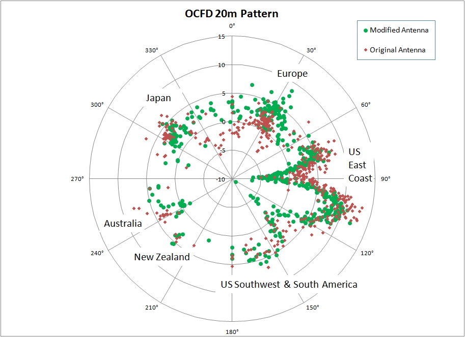
Although the northern performance did improve, the pattern looks less like the model than before. Particularly, the null at 90 degrees got deeper – not expected in the model runs, and the lobe at 105 degrees is still pretty strong. Maybe I didn’t go quite far enough with the change? But definitely there is some improvement, and the ~3-4 dB increased gain northward has helped considerably with contacts into Europe.
Although not perfect, the ability to map a wire antenna, compare with NEC models and then make small modifications can actually lead to significant performance enhancement.
