
A couple of years ago I designed this antenna which had the good property of substantial low elevation gain and the model generated consistent and predictable 4NEC2 results. The wire that it would replace was already “pretty good” so it’s taken two years to decide to build it. But I always had the feeling that I needed to validate the design, so with some nice weather, the time had come.
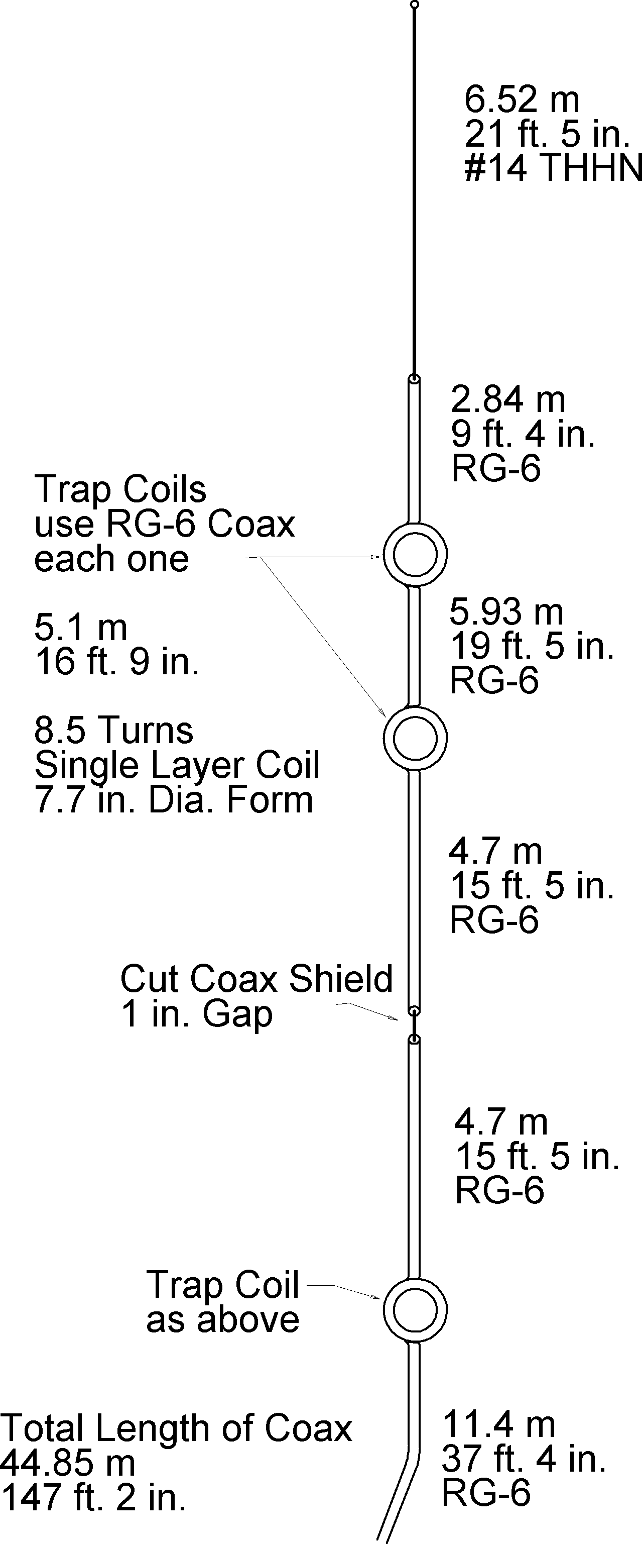
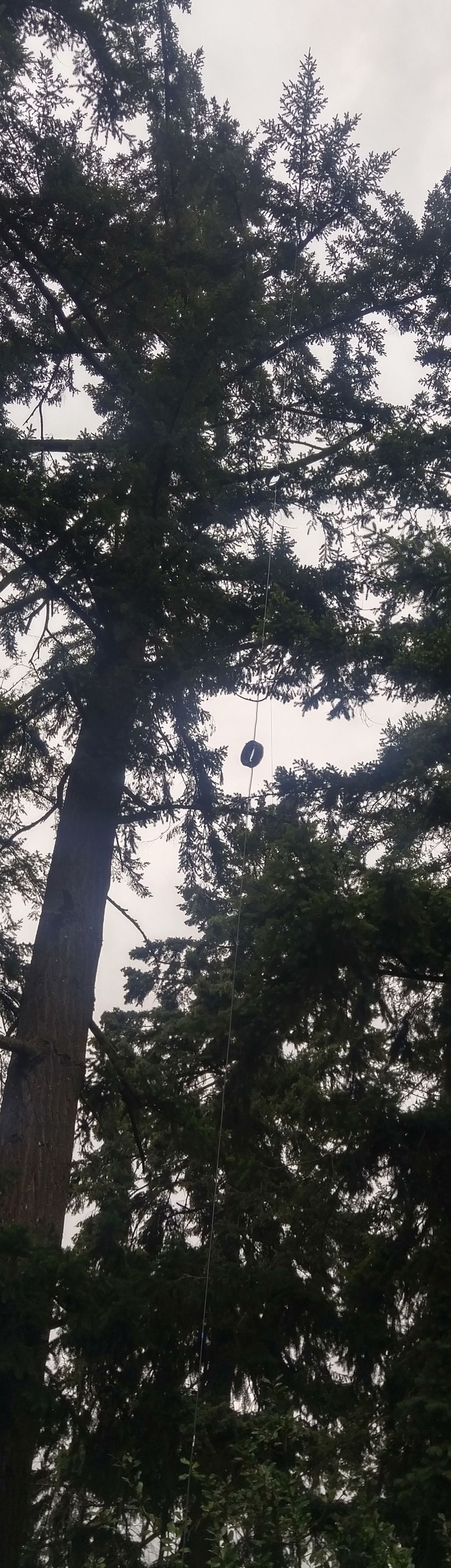
This antenna is a “pull-up” vertical that requires a tall tree. The “old” wire collinear used a very similar feed system. A lower 20m trap inductor had approximately the same overall transmission line length as the the new design, so rather than rebuild it exactly to the new design recipe, I used that section as it was. The figure to the right shows the basic antenna geometry. The table below lists the critical lengths and dimensions of what was built compared to the previously optimized design.
| Design Parameter | As Built | Optimized Design | Units |
| Coax Type | RG-6 | RG-6 | |
| Coax Velocity Factor | 0.83 | 0.83 | |
| Coax Impedance | 75 | 75 | Ω |
| Height | 30 | 30 | meters |
| Length of line between top & bottom dipoles | 17.65 | 23.67 | meters |
| 1.0 | 1.34 | wavelength | |
| L1 Length of top ¼ wave section – #14 wire | 6.83 | 6.52 | meters |
| L2 Length of top lower ¼ wave – RG-6 | 2.84 | 2.84 | meters |
| L3 Length of bottom upper ¼ wave – RG-6 | 5.0 | 4.70 | meters |
| L4 Length of bottom ¼ wave section – RG-6 | 4.72 | 4.70 | meters |
| Lower Trap – coil diameter | 135 | 196 | mm |
| Lower Trap L (calculated) | 22.5 | 18.2 | µH |
| Lower Trap C (calculated) | 5.5 | 7.0 | pF |
| Length of coax for bottom trap | 5.95 | 5.1 | meters |
| Electrical Length of Bottom coax to break | 27.15 (TDR) | 26.6 | meters |
| Electrical Length of Upper coax to break | 28.7 (TDR) | 23 | meters |
| Physical Length of Upper coax to break | 23.7 | 26.6 | meters |
| Lower Trap turns | 14 | 8.5 | turns |
| Length of coax for upper traps | 5.34 | 5.1 | meters |
| Upper two traps – coil diameter | 200 (8″ flower pot) | 196 | mm |
| Upper Trap turns | 8.5 | 8.5 | turns |
| Trap L (calculated) | 18.2 | 18.2 | µH |
| Trap C (calculated) | 7.0 | 7.0 | pF |
| Separation between dipole ends | 5.6 | 5.93 | meter |
| Performance Results | Measured | Model | |
| SWR @ 14.1 MHz. | 1.5 | 1.09 | |
| Gain at 10° elevation | ? | 4.18 | dBi |
| Radiative Efficiency | ? | 57.2 | % |
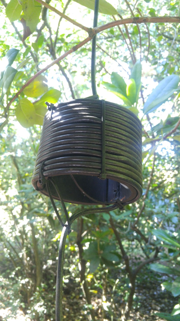
I used an available plastic flower pot as the form for the upper traps. I tried to maintain the dimensions for the active radiator elements and allowed the spacing between the two upper traps to fall where it might after winding the 8.5 turns on each for trap. I divided the cable run into two halves that were joined at the lower feed point. I tuned the electrical length of the upper cable by measuring the electrical length by time domain reflectometry (TDR) using my oscilloscope and a fast pulser. I discovered that my nanoVNA also has a TDR function that can accurately measure the electrical length of cables. Measuring the electrical length eliminates any doubt about the relative velocity factor, Vr, of the cable, and is at least as accurate as using a tape measure and assuming you know what Vr is. The numbers in the table above also reflect some small changes I made to make use of an unexpected resonance for the 30m band and a couple other small changes that resulted from that decision.

A unique feature of this antenna are the self resonant coils of the feed line coax used as traps that defined the ends of the radiating dipoles. Designing the self-resonant coils is its own little sub-problem. I built a trap coil calculator spread sheet that made this calculation easier to deal with. The upper traps use a little less coax and have fewer turns of larger diameter. There is no reason not to make them all the same; I just had the lower one already installed.
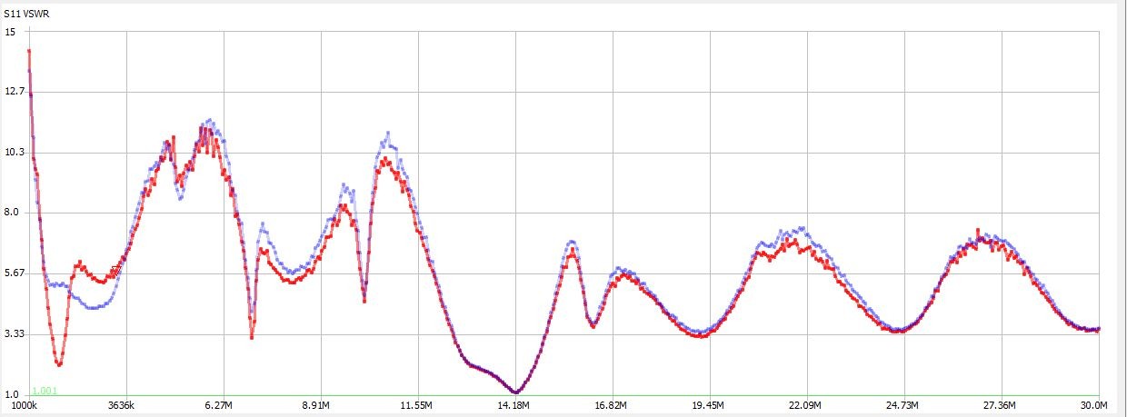
The good news is that the model results were largely verified by the resonance characteristics of the antenna. The modeled and measured SWR tuning curves are shown below.
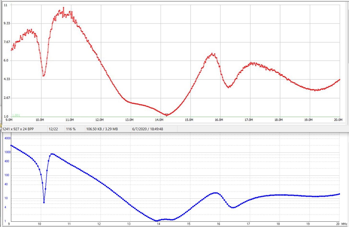
The coils of coax must be acting like traps or we would not get the predicted results. You can see that some of the features of the model are reflected in the measured data. One obvious feature is the sharp resonance at about 10 MHz. I scratched my head over that for a little while until I realized that the length of the transmission line between the two vertical dipoles gives rise to this feature as the wave bounces back and forth in the coax. I chose to tune the length of the upper cable so that the resonances is exactly on the 30m band. This was probably a foolish exercise because the 30m pattern peaks at 30 degrees elevation angle, and much of the energy will undoubtedly just heat the cables, but it seemed like a coincidence that deserved at least a little investigation.
Note that the measured SWR never shows anything above about SWR 10, whereas the model climbs to >1000. The SWR measurement relies on being able to measure the level of reflected signal from the antenna, but the antenna is a very big noise source. Measuring the difference between having the antenna return 98% of the signal compared to 99% of the signal is difficult with a high noise floor, so there is a natural maximum measurable SWR.
The feed from the “old” wire was set up with a ferrite choke on the feed line and a connection to the shield of the coax right above it. That allowed for a connection to an elevated radial so that the vertical could be used on the 160m band. This infrastructure was still in place. The SWR plot across the entire HF region is shown below with and without this 160m radial connected.
Indeed, the antenna can be made to work for the 160m band with the radial. The fancy series feed and trap coils more or less disappear at the low frequency and there is just a tall wire. Above about 3.5 MHz the effect of the radial wire is invisible on the SWR plot. The sharp resonances at about 7 MHz and 10 MHz are associated with the transit time in the cables. Very sharp resonances on the SWR plot mean that the reactive components in the antenna structure are doing a good job of storing circulating energy but the radiative parts of the antenna are not doing such a good job of radiating it away.
This design is optimized for 20m, but there is always the question about what happens if I try to run it on another band. Clearly the traps will no longer work and RF is going to go where I don’t want it. The SWR will be poor, but maybe with a tuner it would work on some bands. The model results for 17m and 15m were the most promising.
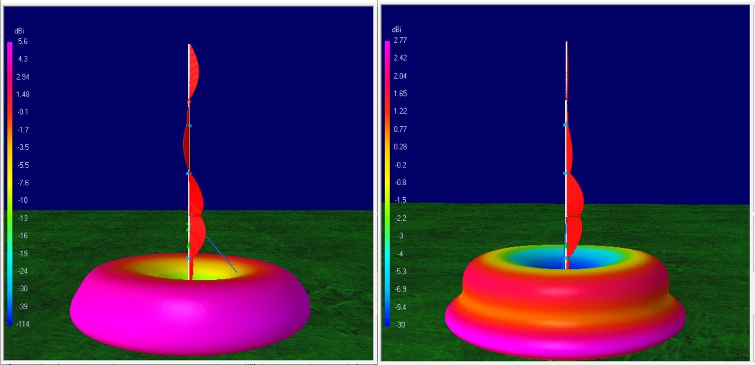
Although the antenna is not at all resonant on 15m, the radiation pattern is very good. Tests using it with a tuner seems to give good preliminary results, but band conditions have not conducive for extensive testing.
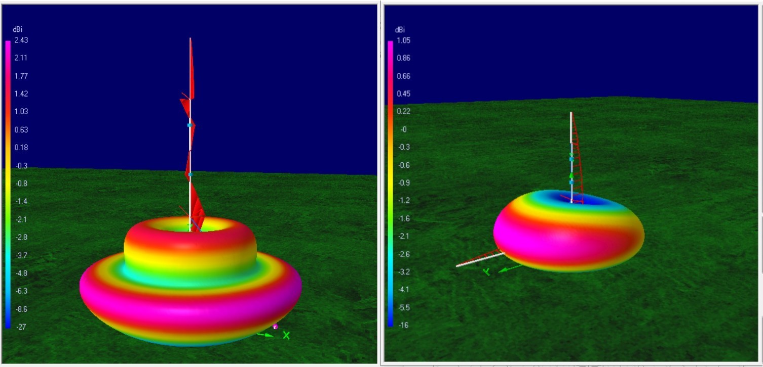
The 30m pattern is looking skyward; little reason to pursue the parasitic resonance there. With a single resonant elevated radial we get a usable 160m pattern. It can be improved by using two radials. With a tall wire in the air, you might as well get 160m while you are at it!
On-air Performance
When I first tested the new antenna on 20m I was disappointed by how much noise there was. This is a characteristic of vertical antennas especially in and around urban environments. It took a while to appreciate that the 360 degree, 4 dBi low elevation gain pattern was allowing the antenna to pick up a lot of noise from all over. WSPR tests confirmed that the antenna can be heard much better than it can hear. A brief band opening into Europe allowed for some FT8 contacts and PSK Reporter signal reports that showed very good signal reports to DX locations. I found that using my high long wire as a receive antenna proved very effective when transmitting on the new collinear.
The best comparison test so far was a simultaneous WSPR run with Dave Cole, NK7Z, and his very nice 6BTV vertical installation. Propagation conditions were only modest during the test so we were mostly looking at US stations, but there was enough data to draw some meaningful conclusions. The best measure of the TX capability of the antenna is to compare the signal reports from simultaneous reception of spots from the two antennas under comparison. Both transmitters were running 2 watt WSPR transmissions.
| Antenna | Total unique reporters | Number TX cycles | Number of simul-taneous TX cycles | Number of simul-taneous TX spots | Average signal report difference | Number of RX cycles | Number RX spots | Ave RX spots/cycle |
| 20m Vert. Collinear | 145 | 37 | 14 | 282 | 2.74 | 176 | 570 | 3.2 |
| 6BTV w/ 40 buried radials | 115 | 44 | 14 | 169 | 411 | 2.4 |
We had 14 occasions when we both were transmitting simultaneously. I used the 282 simultaneous reception reports to make an estimate of the two antennas relative TX gain performance. The average difference signal reports was about 2.7 dB in favor of the collinear. Reception reports also favored the collinear with it receiving an average of 3.2 spots/cycle compare to 2.4 spots/cycle for the 6BTV.
The long spots we both received are listed below. The collinear came out on top here quite clearly as well.
| Call | SNR | Reporter | RGrid | km | # Spots |
| 6BTV Ground Plane Vert. | |||||
| NK7Z | -24 | VK7JJ | QE38lr | 13041 | 2 |
| NK7Z | -21 | TF4AH | HP75rm | 6000 | 1 |
| NK7Z | -21 | VE1VDM | FN85ij | 4613 | 2 |
| NK7Z | -13 | WJ1I | FN41xq | 4253 | 1 |
| NK7Z | -8 | KK1D | FN31vi | 4099 | 1 |
| NK7Z | -23 | W1JS | FN43dc | 4069 | 3 |
| NK7Z | -23 | WA2TP | FN30lu | 4055 | 9 |
| NK7Z | -20 | K4RUR | EL98gp | 4044 | 2 |
| NK7Z | -23 | AA1WH | FN32qd | 4035 | 1 |
| NK7Z | -25 | AI6VN/KH6 | BL10rx | 4007 | 22 |
| Collinear Elevated Vertical | |||||
| AF7NX | -23 | VK7JJ | QE38lr | 13038 | 8 |
| AF7NX | -25 | ZL2BCI | RE79nd | 11275 | 4 |
| AF7NX | -21 | ZL1ROT | RF81cx | 10973 | 1 |
| AF7NX | -19 | EA8BFK | IL38bo | 9209 | 5 |
| AF7NX | -16 | TF4AH | HP75rm | 5999 | 2 |
| AF7NX | -22 | VE1VDM | FN85ij | 4617 | 14 |
| AF7NX | -16 | WJ1I | FN41xq | 4258 | 5 |
| AF7NX | -25 | W1FRV | FN42qb | 4198 | 3 |
| AF7NX | -25 | AA1A | FN42pb | 4191 | 7 |
| AF7NX | -17 | WA9WTK | FN42fk | 4112 | 1 |
| AF7NX | -23 | KK1D | FN31vi | 4105 | 3 |
| AF7NX | -22 | W1JS | FN43dc | 4074 | 9 |
| AF7NX | -23 | WA2TP | FN30lu | 4061 | 16 |
| AF7NX | -23 | K4RUR | EL98gp | 4052 | 6 |
| AF7NX | -20 | AA1WH | FN32qd | 4040 | 12 |
| AF7NX | -22 | KD2AVU | FN30er | 4020 | 7 |
| AF7NX | -21 | WA3098SWL | FM28jh | 4003 | 9 |
| AF7NX | -15 | AI6VN/KH6 | BL10rx | 4003 | 39 |
The collinear antenna received 115 spots compared to 44 on the 6BTV from places more than 4000 km away. One might expect that the collinear would show its best performance on distant stations where low elevation angle performance is most important. It is difficult to make comparisons on a few stations because of confounding statistics, but the Hawaii station that spotted both of us many times was received by the collinear on average 10 dB better than by the ground plane vertical.
