
In this article I discuss getting the three element hex beam to work well. Please see Designing a Three-Element Hex Beam and Building the Three-Element Hex Beam for those phases of this project.
The hex beam is basically a compact Yagi. Like the Yagi, the parasitic elements of the hex beam develop RF currents that are phased appropriately to generate a directional radiation pattern. However, the folded up nature of the hex beam leads to functional and tuning ambiguity. The process I go though here could be used to tune any multielement antenna in conjunction with modeling information that clues you into optimized current distributions.
Yagi Insight
Before we get into the details of our hex beam, lets look at some properties of a simple three element Yagi. I made a NEC model and let the optimizer determine the best length ratios for the reflector and director and the best spacing from the driver for those elements, all normalized to the wavelength. What we discover by this exercise is that the best performance with the standard three element Yagi places the director and reflector a little more than 1/4 wavelength from the driven element. The reflector is about 3.5% longer than the driven element and the director about 3% shorter. We discover that the optimum three element Yagi is a big squarish antenna. You can squeeze the elements together and it will work, but with not quite as much gain. If you try to make the antenna even bigger by spreading the elements even further apart, they don’t couple quite as well to the driven element and again the gain suffers.
The other thing you can look at with a model is the relative phase of the currents on the three elements. The image below shows the Yagi model run results with the current phases on the wires.

The model can tell you the amplitude as well, but the phase on the wires is the key to how the Yagi works. In the above illustration, the driver (yellow) has phase of 0°. The reflector (pink) has a phase of 127° leading the driver. The phase needs to be leading the driver because by the time an EM wave launched from the reflector wire reaches the driver wire, time and phase will have passed. In this case there is about 112° phase spacing between reflector and driver, so waves launched by the reflector and the driver wires will be closely match in phase for an EM wave traveling in the forward direction at the speed of light. Similarly, the director wire needs to lag the driver, seen here by 162° whereas the physical space is about 95° – not as close but still adding in the forward direction to the total. We will keep this model in mind as we try to make the three element hex beam work.
Tuning
The journey between a good antenna model and a good working antenna can be a torturous one. The path is more twisted the more complicated the antenna is. With a dipole you have just one parameter, just the length of the wire. With an off-center-fed dipole, you have two parameters, the length and the feed point offset. The first antenna I built that had serious optimization challenges was my multi-band big wire, with half a dozen free parameters. If we step up to the three-element multi-band hex beam, all of a sudden we find 7 parameters for each of the wire sets for the 5 bands of the hex, plus another 3 or four parameters for the trapped “draped dipole” for 30/40m bands. Add couple for the feed point at the antenna and the length of the coax feed and that is a total of about 40 parameters which were either fixed as constraints or determined by model optimization to describe the antenna geometry. Fortunately you do not need to find all of them all at once. The wires for one band only minimally affect the other bands.
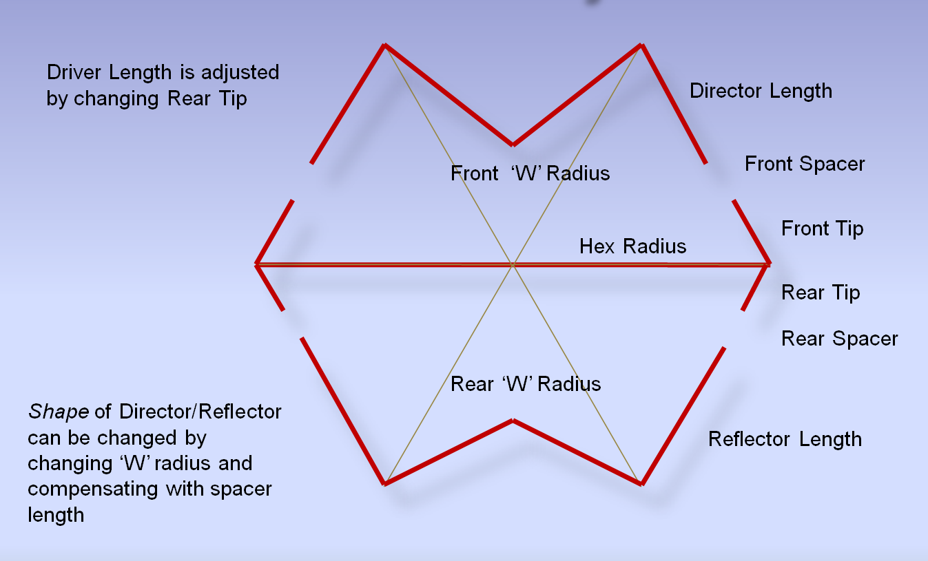
The figure above shows the typical 3-element hex wire set. The model gives us numbers for everything, so if we build it by the recipe you might expect it just to work. But in the real world with gravity that makes the wires sag, bamboo of varying stiffness, dozens of measurement errors that accumulate, and the constraints of a “sprung” tension structure, you will invariably need to make adjustments to regain “tune.” With your best guesses you make a start and measure the tuning curve.

The figure above shows an early ragged tuning curve on the entire antenna before much tuning was attempted. Tuning up the 40m/30m dipole was fairly straightforward adjustment of the lengths of the wires before and after the trap. I then started with the 20m band and attempted to tweak the wires to improve the SWR plot. It became clear that for the three-element wires, you could figure out which wire was the best one to adjust based upon how you need to change the SWR about the band.

The longer reflector wire sets the lower portion of the band, the director wire mostly affects the upper portion and the driver is best tune to the middle of the band for low SWR. Making small adjustments with the wires, one at a time, using this guidance you can make progress. But a good looking SWR plot alone is not enough to guarantee good performance. Comparison with my trusty standard two-element hex showed that you could have good SWR but poor forward gain and directivity.
The 17m band was particularly tricky. I am not expecting dramatic improvements over the two-element hex for any of the bands above 20m, but I don’t want to go backwards! At some point in this process frustration kicked in and I needed more information – namely phase. For this part of the process I built a pair of current sensor that I could place on the wires so I could measure the real-time currents on the driver and compare to current on the parasitic elements. I also asked my model to tell me what I should expect to happen to these currents under various amounts and methods of miss-tune.


The charts above show what the model says should happen if one of the antenna elements is mistuned by various amounts. It also show the optimized parameters for the hex beam (gray rows), and an optimized three-element Yagi (bottom row, top chart). The hex beam is a smaller antenna than the Yagi with the average position of the reflector and director closer to the driver. Hence the relative phase shift between driver and parasitic elements is smaller for the hex beam. With the Yagi elements further away from the driver they are not excited as hard as for the hex beam so the normalized current amplitudes are also less.
What I was most interested in was how the phase shift changes as you mistuned the parasitic elements. Notice that as you mistune the reflector (green) or director (red) element length, the phase on the mistuned element changes monotonically in a predictable way. You can accomplish the mistune either by changing the wire length of the parasitic elements, or by changing how the wire is stretched on the hex structure as shown in the second chart.
To use this information to help us reach a better tune of the antenna, we need to measure the relative phase on the antenna wires. The most direct way to do this is with a current transformer on the wires. I built three identical sensors which I describe more fully here and three identical length coax runs so that it was possible to directly monitor the currents on all three wire elements simultaneously on an oscilloscope.
The images below show the current sensors set up for cross calibration purposes on the driver wire. The signals are within 2% and in-phase with one another when 5 Watts is supplied to the antenna.

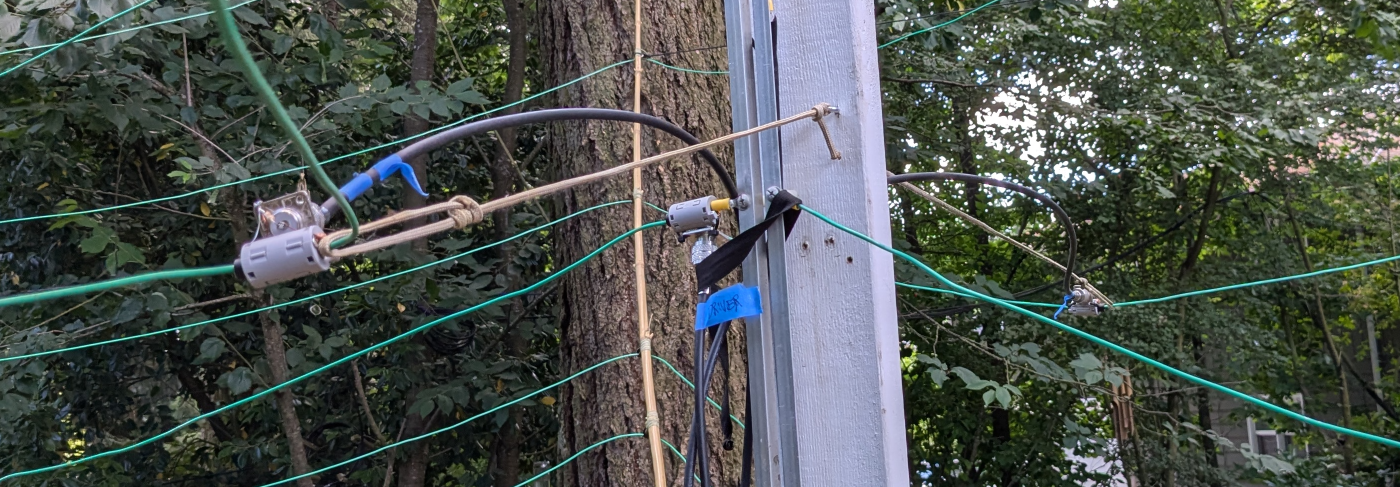
The signal cables for the sensors were run along the low-side feed-line (connected to shield of the feed line cable) and then radially out from the center support to near the center of the wire element being measured. This way there should be very little coupling between the driven RF and the probe cables. The SWR curve did not perceptively change with or without the probes on the wires, suggesting that they indeed did not change the antenna behavior. The photo below shows the sensors on the three elements of the 15m wires.
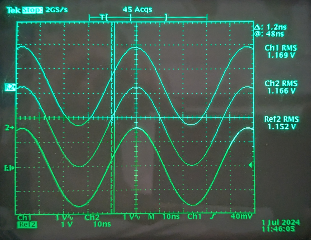
If you are patient and lucky, you can eventually get the signals on the sensors to look something like in the photo below. The driver is the lower trace; the upper two traces are the reflector (leading), and the director (lagging), the driver with phase shifts near 90 degrees and similar amplitudes.

What one discovers is that it is pretty easy to move the phase around with small adjustments to the wires. I won’t say getting there is easy — just that it is possible. I was happy to be able to lower and raise the antenna in just a few minutes because I did this dozens of time in the tuning process. The phase measurement and SWR measurement offer two complimentary ways of getting at the band tune. The phase measurement can accurately guide you to the optimum length for the parasitic elements. Low SWR is the best measure for adjusting the driver. But everything interacts, so you have to go around the circle a time or two.
If I had a method it was this:
• Start with the model recipe
• Use SWR sweep to check band resonance
• Make small adjustments to elements one at a time
• Verify phasing with current probes as needed – usually needed
• Keep antenna shape ‘relaxed’ in this process so it will reliably return to the same shape when deployed.
• Rinse and repeat! Antenna up and down dozens of times.
Merely using the SWR plot proved to be an unreliable metric. It is possible to have a good looking SWR plot across the band but have the antenna fire backward.
The figure below shows the present 7-band SWR tuning curve for the antenna.

One thing to notice are the steeper sides on the three-element bands compared to the 30/40m dipoles. All of the three-element bands were adjusted with the help of the current probes with the exception of the 10m band, which I had not yet optimized.
Performance
Proof of the pudding are quantitative comparisons against my venerable two-element hex beam that this new antenna is destined to replace. To make these measurements I use my ALLPLOT software and simultaneous FT8 signal reports from both the old two-element hex beam and the new three-element hex beam, data collected over the period of a day or so. I use the two identical receivers in the RSPduo SDR, with both filters and internal gain settings identical. A good result is shown below.

Both antennas were pointed 20° N from my station in Oregon, more or less toward Europe. Red means the 3EL hex is preferred, blue means the 2EL hex is better. You can see the strong enhancement of the 3EL over the 2EL into Europe and the the commensurate rejection in the backward direction with the New Zeeland stations. In the forward direction the 3EL hex is providing the ~3 to 4 dB gain improvement we were hoping to get on the 20m band.
The antenna has been up for over a year now, and continues to outperform many of my DXer friends Yagis and hexes, for whatever reason. The effort to get the complex antenna tuned has been very much worth the performance it now delivers. The HF bands 40m through the 10m band all come in on a single cable and no tuner is required to work any of these bands.
